CarND Project 3: Behavioral Cloning
Writeup Template
The goals / steps of this project are the following:
- Use the simulator to collect data of good driving behavior
- Build, a convolution neural network in Keras that predicts steering angles from images
- Train and validate the model with a training and validation set
- Test that the model successfully drives around track one without leaving the road
- Summarize the results with a written report
Rubric Points
Here I will consider the rubric points individually and describe how I addressed each point in my implementation.
Files Submitted & Code Quality
1. Submission includes all required files and can be used to run the simulator in autonomous mode
My project includes the following files:
| file | description |
|---|---|
model.py |
containing the script to create and train the model |
helpers/data.py |
helper module to handle data wrangling |
helpers/augment.py |
helper module to augment training data on the fly |
model.h5 |
containing a trained convolution neural network |
drive.py |
for driving the car in autonomous mode |
video.mp4 |
video recording of autonomous mode using my model model.h5 on track 1 |
README.md |
project writeup |
While developing and training I used Python 3.5.2 with Keras 2.0.2 and TensorFlow 1.0.1.
2. Submission includes functional code
Using the Udacity provided simulator and my drive.py file, the car can be driven autonomously around the track by executing
python drive.py model.h53. Submission code is usable and readable
The model.py file contains the code for training and saving the convolution neural network. The file shows the pipeline I used for training and validating the model, and it contains comments to explain how the code works.
Training Data
1. Collection
Due to a lack of confidence in my car simulator driving skills, which are based on experience with 3D racing games, I immediately opted for the training data provided by Udacity. Later on, I decided to practise my simulator driving skills and record some more data to extend the provided data set with some curvy driving and also with recovery driving.
2. Analysis
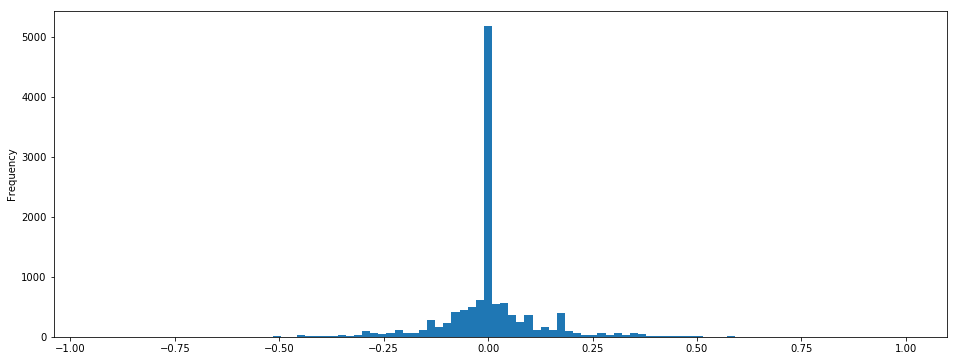
A first look at the data provided by Udacity reveals that in includes by far more straight-ahead driving (steering angle around 0.0) than left/right steering. That's when I decided to collect my own data additionally, as track 1 does not have that many straight sections. I drove on track 1 in both directions.
After adding my own recordings, the data now looks as follows:
| steering direction | count |
|---|---|
| left (angle < 0) | 3883 |
| right (angle > 0) | 3740 |
| straight (angle = 0) | 4420 |
There are 12,043 data points in total.
Here's a histogram of steering angles including both my own and Udacity's training data:
There's still disproportionately more data for driving straight-ahead.
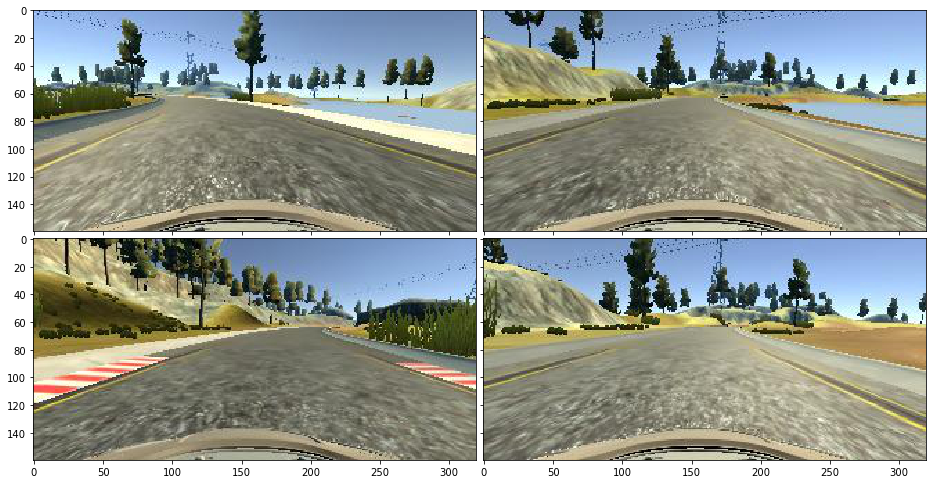
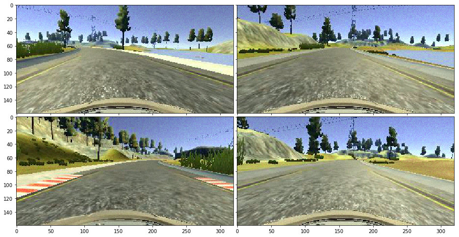
The input images have the size 160 x 320 x 3. Here are 4 sample images:
3. Preprocessing
Data Augmentation
Due to the high amount of data with steering = 0 I decided to randomly drop that data from the training data. Additionally, in order to increase the overall amount of training data and make the model more robust and generalized, I decided the augment the data in several ways (see helpers/augment.py, lines 32-62):
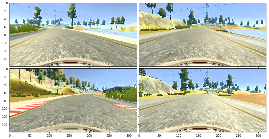
- change brightness of input image
- this helps the model generalize beyond brightness/darkness of a scene
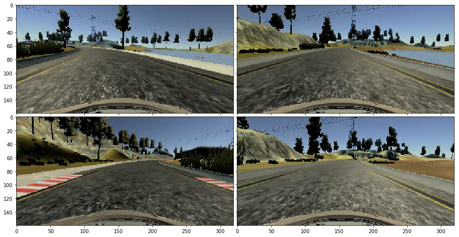
- add random noise to input image
- this helps generate non-identical training images for the same steering angle
- flip input image of center camera
- this helps increase the amount of training data for left/right steering
Flipping is additionally applied to brightnened/darkened images as well as images with added noise.
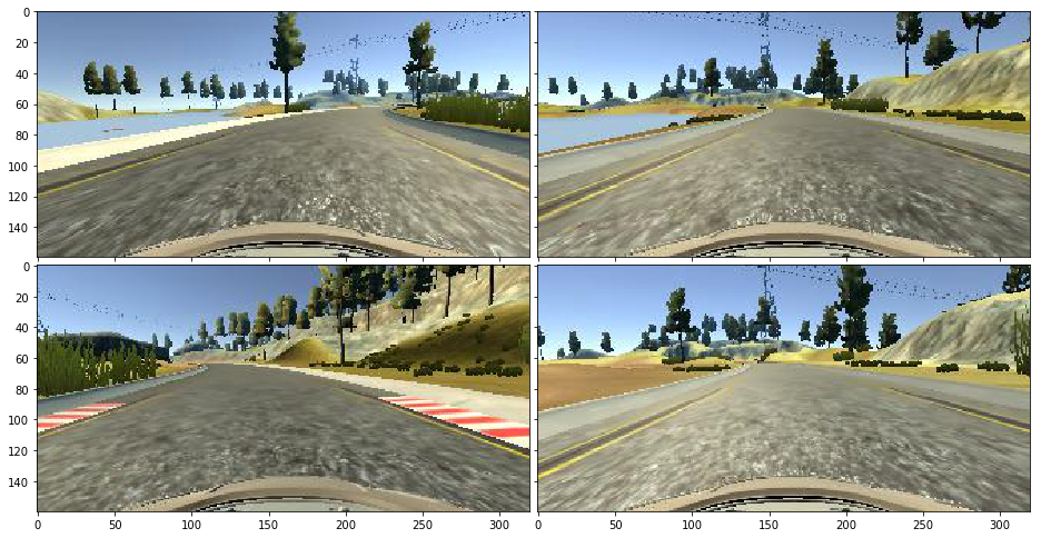
Here are the various augmentations applied to the above sample images:
Brightened
Darkened
Added Noise
Flipped
Actual Preprocessing
I decided to pass the images into the model in HSV color space as this not only simplifies modification of brightness but also, to me, seems like a more 'semantic' format.
Besides transformation into HSV, all further preprocessing is done within the model.
The first layer of the model crops the image, thereby removing the part of the image above the horizon (i.e. sky) and the lower part including the hood of the car. I remove both because the hood is a constant, never changing part of the image, which provides no additional valueable information. For the same reason I also crop the sky as it keeps changing, but obviously does not determine the steering angle. Cropping also reduces the input size of the model, therefore reducing it's number of parameters and computation needed for training.
The second layer normalizes the input image of dimension 74 x 320 x 3 from integer values ranging between 0 and 255 to floating point values between -0.5 up to 0.5 (model.py, lines 32).
Model Architecture and Training Strategy
0. Model choices
Having learned about some existing neural network architectures in previous lessons, I wanted to give the NVidia model a try. All of my training was done on my personal laptop, which has an NVidia GPU with 2GB of RAM. This, however, turned out to be a bottleneck when a model grew too big. Training the NVidia was doable, albeit quite slow and memory hungry. I then thought that the NVidia model was too potent for this task and tried to come up with a smaller, hence faster model.
1. An appropriate model architecture has been employed
Out of the motivation of being able to train the network on my local GPU with just 2GB of RAM, I tried to design a smaller neural net than the NVidia one. (see model.py, lines 44-56)
In order to achieve that, I aimed to reduce the data size early on by using an 8 x 8 convolutional layer with a stride of 2, followed immediately by a max pooling layer of size 2 x 2. Then, one convolution of 5 x 5 is followed by three convolutions of 3 x 3 before flattening the data, applying a high dropout of 0.6 (60% of the data is lost) and passing it to 3 fully connected layers. The last single-neuron layer determines the output. Each convolutional and fully connected layer (except for the output layer) uses ELU as an activation to introduce non-linearity. As mentioned before, data normalization is done in the second Keras Lambda layer (see model.py, line 32).
Below is the output of the Keras model.summary():
Layer (type)                 Output Shape              Param #
=================================================================
cropping2d_1 (Cropping2D)    (None, 74, 320, 3)        0
_________________________________________________________________
lambda_1 (Lambda)            (None, 74, 320, 3)        0
_________________________________________________________________
conv2d_1 (Conv2D)            (None, 34, 157, 12)       2316
_________________________________________________________________
max_pooling2d_1 (MaxPooling2 (None, 17, 78, 12)        0
_________________________________________________________________
conv2d_2 (Conv2D)            (None, 7, 37, 24)         7224
_________________________________________________________________
conv2d_3 (Conv2D)            (None, 5, 35, 32)         6944
_________________________________________________________________
conv2d_4 (Conv2D)            (None, 3, 33, 32)         9248
_________________________________________________________________
conv2d_5 (Conv2D)            (None, 1, 31, 32)         9248
_________________________________________________________________
flatten_1 (Flatten)          (None, 992)               0
_________________________________________________________________
dropout_1 (Dropout)          (None, 992)               0
_________________________________________________________________
dense_1 (Dense)              (None, 256)               254208
_________________________________________________________________
dense_2 (Dense)              (None, 64)                16448
_________________________________________________________________
dense_3 (Dense)              (None, 16)                1040
_________________________________________________________________
dense_4 (Dense)              (None, 1)                 17
=================================================================
Total params: 306,693.0
Trainable params: 306,693.0
Non-trainable params: 0.0
_________________________________________________________________
In total there around about 306,693 trainable params. This is considerably less than the NVidia model, which had 559,419 trainable params, which results in higher memory consumption and more computation needed to train the model. Consequentially, the NVidia model requires more training data. With the smaller 66 x 200 x 3 input size the NVidia model assumes, Keras reports Trainable params: 252,219.0.
2. Attempts to reduce overfitting in the model
The model contains a dropout layer in order to reduce overfitting (see model.py, line 52).
On top of that, I recorded my own driving in the simulator, in order to add more heterogenous data.
For training and validation the data was split (see model.py, line 88).
3. Model parameter tuning
The model used an adam optimizer, so the learning rate was not tuned manually (see model.py, line 37).
4. Appropriate training data
Training data was chosen to keep the vehicle driving on the road. I used a combination of center lane driving and recovering from the left and right sides of the road in my own recorded data. Additionally, I used the left and right camera images with a steering angle correction of ±0.25 to simulate recovery.
Model Architecture and Training Strategy
1. Solution Design Approach
As mentioned above, my first step was to use the NVidia model as described here, because it was employed to solve the same kind of steering angle prediction as in this project.
I quickly came to the conclusion that the NVidia model was exhausting my GPU with just 2GB RAM, so I decided to try to come up with a leaner model architecture, which would still be able to do the job.
I took the NVidia model and tried to reduce its size / number of trainable parameters.
The NVidia model takes 66 x 200 x 3 input images. this differs from what the simulator provides. Even after cropping, the remaining image still has 74 x 320 x 3 pixels. I tried to resize/scale the input within a Keras Lambda layer, but gave up that idea as the results were not as good as with the full size input. Similarly to the NVidia model, my model starts with a large convolutional layer. Instead of 5 x 5 I decided to use an 8 x 8 kernel in the first convolution due to the larger input image size. Before reaching the fully connected layers, my model's internal data passed to the fully connected layer has the dimension 1 x 31 x 32 (= 992), which is a roughly comparable amount of information the NVidia model retains with a dimension of 1 x 18 x 64 (= 1152).
In order to gauge how well the model was working, I split my image and steering angle data into a training and validation set. I found that most of the time my first model had a low mean squared error on the training set and an even lower mean squared error on the validation set. What was irritating for me was that the accuracy measure provided by Keras was nowhere near where I had expected it. I therefore spent a lot of time trying to debug a problem that wasn't even there. From the start I had hope to achieve an accuracy of above 0.8, even above 0.5 would've been encouraging. Most of my trained models were usually in the 10-27% range, which was confusing. I then tried running them in the simulator and found out that even seemingly low accuracies yielded and acceptable autonomous driving result. Even a ridiculously low accuracy below 1% yielded a safe center-of-lane driving for most of track 1, although eventually going off road at a later stage. The best model I trained had a MSE of below 0.1.
At first I focussed mostly on the model architecture but soon realized that the driving data from Udacity was strongly biased towards straight-ahead driving. As a symptom, early simulator runs often resulted in only very reluctant and low steering angles with the car driving off track at the first bend of the road. I managed to fix that by comparatively reducing the amount of straight-ahead driving in the training data. I drop straight-ahead steering data points with a probability of 80%, i.e. keep only 20%. In order to generate more training data overall, after dropping some of the straight driving, I augment the images by flipping, changing brightness and adding pixel noise. That resulted in the model being more 'confident' in bends and steering appropriately.
At the end of the process, the vehicle is able to drive autonomously around the track 1 without leaving the road. Sadly, my model constantly fails on the narrow leftward bend atop of the first hill after driving surprisingly well. I plan on working to improve the model's track 2 performance as well.
2. Final Model Architecture
The final model architecture (see model.py, lines 44-56) consists of a convolution neural network with the following layers and layer sizes:
| Layer | Description | Input Shape | Output Shape |
|---|---|---|---|
| Cropping | crops the sky and car's hood | 160 x 320 x 3 | 74 x 320 x 3 |
| Normalization | normalizes the input values to a range of -0.5 to +0.5 |
74 x 320 x 3 | 74 x 320 x 3 |
| Convolution | convolutional layer with kernel size 8x8 and strides 2x2 |
74 x 320 x 3 | 34 x 157 x 12 |
| Activation | ELU activation layer | 34 x 157 x 12 | 34 x 157 x 12 |
| Max Pooling | max pooling layer with pool size 2x2 |
34 x 157 x 12 | 17 x 78 x 12 |
| Convolution | convolutional layer with kernel size 5x5 with strides 2x2 |
17 x 78 x 12 | 7 x 37 x 24 |
| Activation | ELU activation layer | 7 x 37 x 24 | 7 x 37 x 24 |
| Convolution | convolutional layer with kernel size 3x3 with strides 1x1 |
7 x 37 x 24 | 5 x 35 x 32 |
| Activation | ELU activation layer | 5 x 35 x 32 | 5 x 35 x 32 |
| Convolution | convolutional layer with kernel size 3x3 with strides 1x1 |
5 x 35 x 32 | 3 x 33 x 32 |
| Activation | ELU activation layer | 3 x 33 x 32 | 3 x 33 x 32 |
| Convolution | convolutional layer with kernel size 3x3 with strides 1x1 |
3 x 33 x 32 | 1 x 31 x 32 |
| Activation | ELU activation layer | 1 x 31 x 32 | 1 x 31 x 32 |
| Flatten | flattening layer | 1 x 31 x 32 | 1 x 992 |
| Dropout | dropout layer with drop rate 0.6 |
1 x 992 | 1 x 992 |
| Fully Connected | fully connected layer | 1 x 992 | 1 x 256 |
| Activation | ELU activation layer | 1 x 256 | 1 x 256 |
| Fully Connected | fully connected layer | 1 x 256 | 1 x 64 |
| Activation | ELU activation layer | 1 x 64 | 1 x 64 |
| Fully Connected | fully connected layer | 1 x 64 | 1 x 16 |
| Activation | ELU activation layer | 1 x 16 | 1 x 16 |
| Output | output layer | 1 x 16 | 1 x 1 |
3. Creation of the Training Set & Training Process
To capture good driving behavior, I first recorded two laps on track 1 using center lane driving. Here is an example image of center lane driving:
I then recorded the vehicle recovering from the left side and right side of the road back to center so that the vehicle would learn how to get back to the center of the road. These images show what a recovery looks like:
The car starts off at the right border of the road:
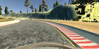
It then progresses towards the middle of the road:
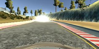
Until the center is finally reached and preserved:
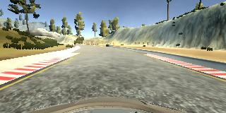
In order to challenge myself, I did not record any data on the second track. Considering how my model currently performs on track 2, I plan on improving that and plan to record data from track 2 as well.
To augment the data set, I also flipped images and angles thinking that this would increase the number of curve driving data to learn from. For example, here is an image that has then been flipped:
More details about the data augmentation I applied and more sample images can be seen above.
After the augmentation, I randomly shuffled the data set inside the generator. I used 20% of the data for validation.
I used this training data for training the model. The validation set helped determine if the model was over or under fitting. The ideal number of epochs was 3-4 as the mean squared error only changed marginally after that. I used an adam optimizer so that manually changing the learning rate wasn't necessary.
