This project is a continuation of the Backyard Flyer project where we executed a simple square shaped flight path. It integrates techniques to plan a path through an urban environment. Check out the project rubric (original link) for more detail on how this implementation is differing from the starter code forked off the original repo.
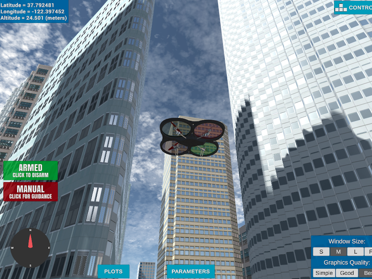
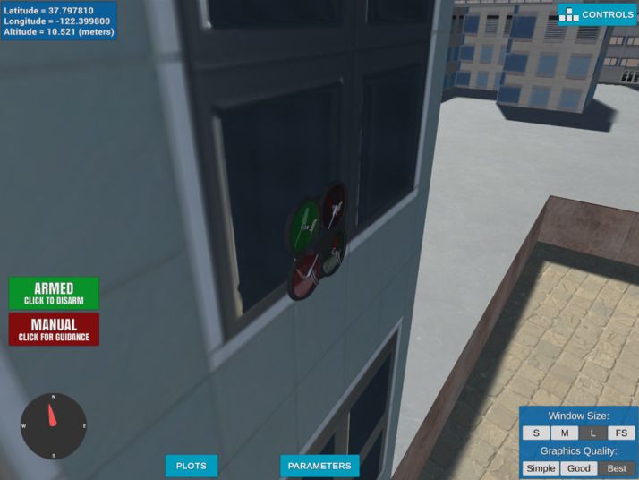
As of version 0.1.0 and 0.1.1, the Udacity-provided simulator is broken on Linux (at least on Ubuntu 18.04, 20.04, but reportedly on some Windowses as well). Once you load the scene, a building is spawned right on top of your drone. Every move immediately results in a crash, which throws off the physics. There's a multitude of reports, some of them you can find here:
- udacity/fcnd-issue-reports#392
- Udacity Knowledge: Is the drone supposed to spawn inside a building? (Spoiler alert: no.)
- Udacity Knowledge: How to change the spawn location of the drone in Simulator? (Spoiler alert: you can't.)
This project is running in a simulated environment. You can download the Linux version of the simulator from from the releases of the sunsided/fcnd-notebooks GitHub repo.
The code was implemented against the Conda environment described in environment.yml. To recreate the environment,
run
conda env create -f environment.ymlAfter that, activate it using
conda activate udacity-fcndStart the simulator and select the Motion Planning scene. Once the scene is initialized, execute the Python code by running
python motion_planning.pyNote that the file backyard_flyer.py is the solution to the Backyard Flyer
project and is meant to be run against the Backyard Flyer simulator scene.
It is kept here for reference, as the project rubric requires it.
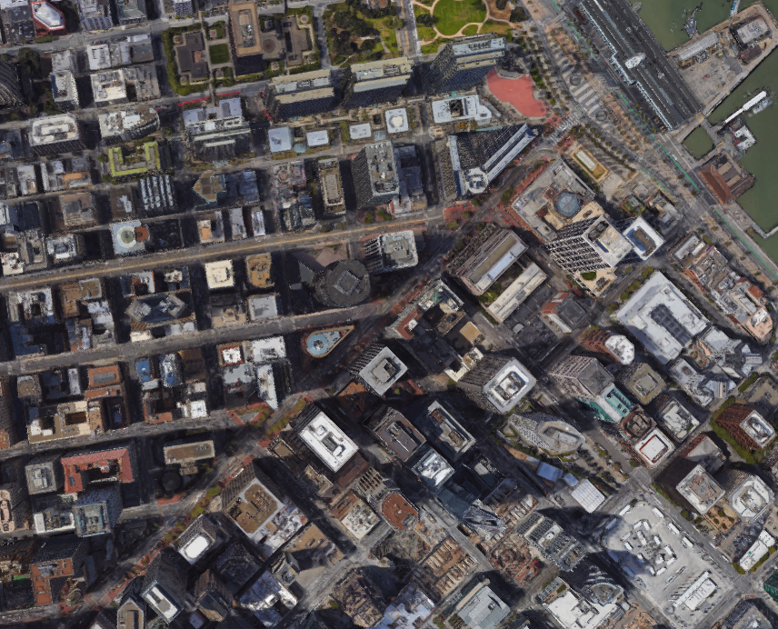
The simulator scene is modeled after Downtown San Francisco with the
starting location somewhere around Market Street
(map code QJV3+57). Here's an aerial picture of the environment:
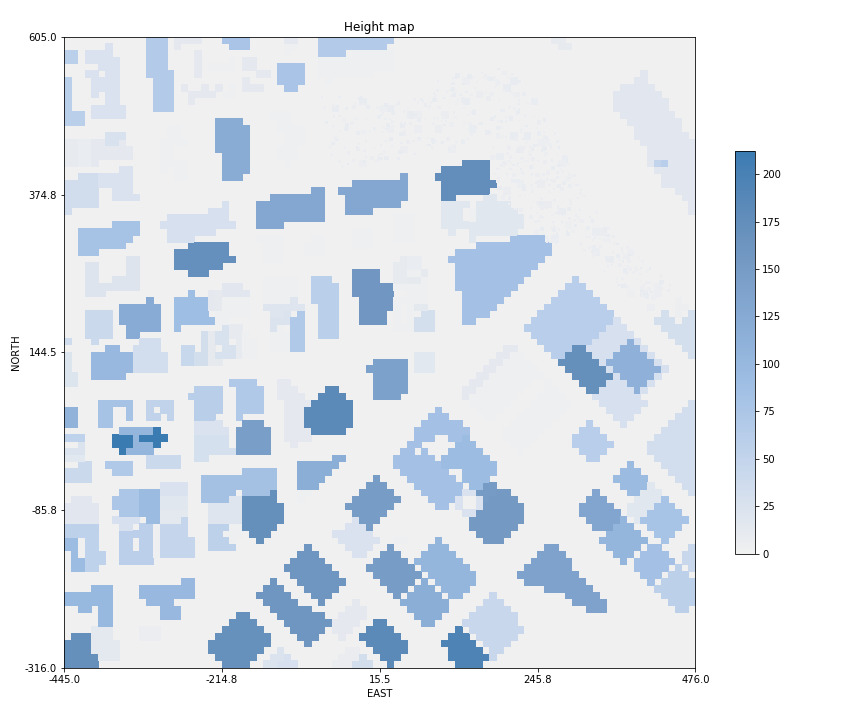
As far as the planner is concerned, the map is initially discretized into a grid. With height information added in, it looks like this:
Note that the height scale in this plot is dimensionless
(no specification is available for colliders.csv), but can
be assumed to be in meters.
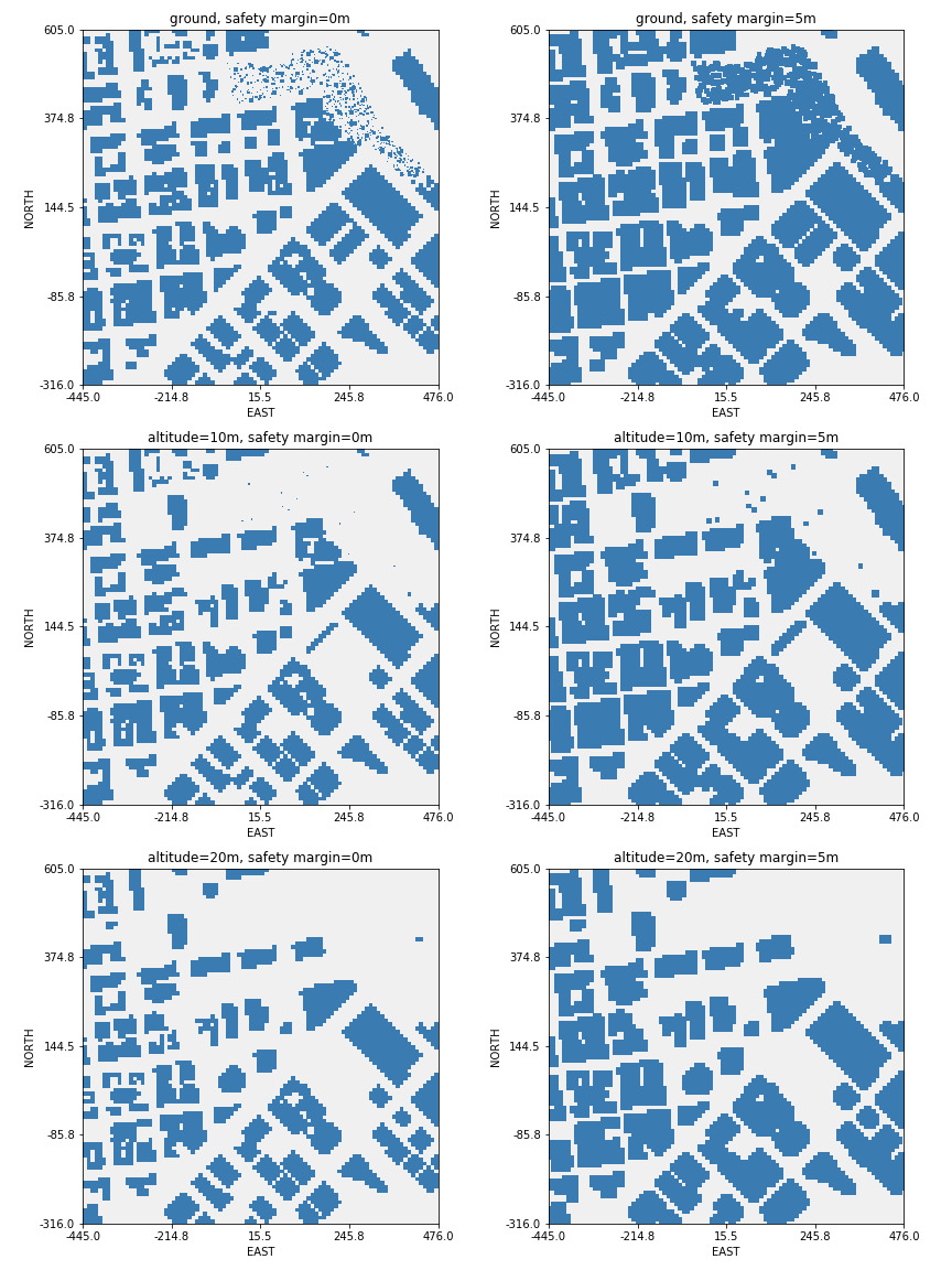
During discretization, we are free to choose any minimum flying altitude, as well as any safety margin to obstacles such as buildings and trees. The following picture shows different variations of the altitude (0m, 10m and 20m), as well as the safety margin (5m and 10m); in these plots, bright spaces resemble safe areas to fly, whereas darker blue areas resemble inadmissible areas:
Note that the maps above are generated from the Udacity-provided colliders.csv file, which
is broken. This will be discussed in detail below; for brevity, here's an augmented
height map (limited at 25 meters of altitude for display reasons) that addresses some of the issues.
As mentioned above, motion_planning.py is based on the backyard_flyer.py solution
which, itself, involves taking off, flying a square, then landing safely.
As before, waypoints are calculated exactly once in the beginning of the mission.
In both solutions, they are issued individually by calling the Drone class' cmd_position(north, east, altitude, heading);
here however, we're now sending off an entire list of waypoints in addition for visualization
by calling send_waypoints(). This, in turn, makes use of a somewhat undocumented
functionality of the underlying MAVLink connection.
What used to be calculate_box() in the Backyard Flyer was now replaced with plan_path().
For this, an extra state PLANNING was introduced in the States enum, to be executed between
ARMING and TAKEOFF.
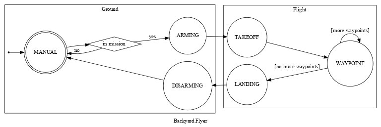
Specifically, the backyard_flyer.py solution code has these state transitions:
For comparison, state transitions of the motion_planning.py starter code look like this:
In plan_path(), first a target altitude and safety margin from obstacles is defined.
We then load the environment from colliders.csv and discretize it using create_grid().
A goal position is generated in ~14m distance (10m to the north and east), then the A*
algorithm is used to plan a path from start to goal (a_star() method), where the heuristic
is implemented using the Euclidean distance.
However, the starter code implementation of the planner is constrained to vertical and
horizontal motion like so:
class Action(Enum):
    WEST = (0, -1, 1)
    EAST = (0, 1, 1)
    NORTH = (-1, 0, 1)
    SOUTH = (1, 0, 1)
(Note that the actions are (north, east, cost) rather than (x, y, cost).)
As a result of this constraint, the generated path moves along the grid cells in a zig-zag pattern.
The following output of motion_planning.py when run off-the-shelf (as of commit bb51472b) gives
a nice overview of the general process. Note that some lines were removed for brevity.
Logs/NavLog.txt
starting connection
arming transition
Searching for a path ...
global home [-122.39745   37.79248    0.     ], position [-122.3974494   37.7924801    0.152    ], local position [ 0.02221821  0.05091386 -0.15224203]
North offset = -316, east offset = -445
Local Start and Goal:  (316, 445) (326, 455)
Found a path.
Sending waypoints to simulator ...
takeoff transition
waypoint transition
target position [0, 0, 5, 0]
waypoint transition
target position [0, 1, 5, 0]
waypoint transition
target position [1, 1, 5, 0]
waypoint transition
... etc. ...
target position [9, 10, 5, 0]
waypoint transition
target position [10, 10, 5, 0]
landing transition
disarm transition
manual transition
Closing connection ...
Some changes were made to the state machine of the starter code in order to separate the different concerns a bit better:
- Instead of directly going from
MANUALtoARMINGstate, we're "downloading" (from CSV) and preparing the map first inDOWNLOAD_MAP_DATAandBUILD_MAP. This is to resemble the fact that obtaining and pre-processing the map is, or can be, an offline process. - The former
PLANNINGstep has been broken into two parts,INIT_MISSIONandPLAN_MISSION_GOAL. This is needed because our entire mission may consist of many sub-goals, such as picking something up in some location and dropping it off somewhere else. The planner only every generates plans up to the next mission goal. - In the starter code, the
WAYPOINTstate would transition intoLANDINGif no more waypoints were available. Now, the planner is instead asked to provide new waypoints if more mission goals remain.
Note that parts of the planning process are executed on the ground as well as in air. In any case, the drone is armed. While it does not make much of a difference in the simulator, arming the drone after planning (and potentially de-arming it before entering the re-planning phase) may give a human operator or bystander the false impression that the device is safe to approach while it is still in planning state. Since the drone is taking off immediately after generating a plan, such a behavior might very well lead to injuries.
Because of that, the drone is armed first (add some warning lights for good measure), even though planning for the next goal might take a while.
As far as the starter code is concerned, the Drone starts its life in the center
of the loaded map and then navigates from there. This holds true for the
simulator, but doesn't in reality. To emulate the behavior of being localized in
the real world, initial coordinates are loaded in receive_and_set_home_position()
from the first line of colliders.csv:
lat0 37.792480, lon0 -122.397450
In here, lat0 encodes the position latitude of 37.792480 degree north
and a longitude of -122.397450 degree east (where negative east, by definition, is west).
As mentioned above, this locates us right here
within San Francisco in the real world (map code QJR3+X2).
The coordinates obtained this way are then set as the drone's home position
via a call to set_home_position(). We can use this information later on
in combination with the grid boundaries of the map to accurately position
us in any grid cell.
Local coordinates are then calculated from the current geodetic coordinates (latitude,
longitude, altitude; this was a required point according to the project's rubric)
and compared to the values provided by the Drone class in determine_local_position().
A couple of interesting goal positions were selected by flying around the map in the simulator; you can find a description and visualization in LOCATIONS.md.
Thinking of these positions, there are some ideas that might be built into a path planner:
- Flying in high altitudes might be dangerous within cities: If for some reason the drone loses control, it might plummet to the ground, possibly injuring someone. As such, staying at low altitudes should always be cheaper than going (too) high. This requires the planner not only to know the map, but also the remaining resources such as battery power (since every positive rotor acceleration causes current to spike, going up and changing directions is naturally more expensive than going down or in a straight line).
- Flying too close to the ground is dangerous as well; because of that, the planner should use a higher cost for all paths outside an altitude "sweet spot" (or range).
- A bit esoteric, but flying over buildings with a flat roof might be wished for if the drone is already at a higher altitude, as the probability of hurting someone in case of an accident may be reduced.
As of the starter code, the provided A* planner only supported horizontal
and vertical movement. Diagonal movement was added with a cost of sqrt(2).
What struck me as odd is how terribly bad the A* implementation performed
even with only four actions on a 2-dimensional grid. Running a performance
analysis showed that most of the algorithm's time is spent in calls to
the heuristic() function and the put() operation of the PriorityQueue class.
The heuristic() itself only called out to np.linalg.norm() for the Euclidean distance.
What's peculiar is that running the A* algorithm in an isolated environment
(astar_performance.py) with identical inputs proved that it is, as would be
expected, extremely fast; in there, only about 140 ms are spent on planning
the path to the first goal (as opposed to 5+ seconds when using the simulator).
Replacing PriorityQueue with the heapq module (a min heap implementation),
the time spent on putting an item into the queue now diminished. Similarly,
replacing the call to np.linalg.norm() with the hand-crafted version shown here
def heuristic(position: GridPosition, goal_position: GridPosition) -> float:
    dx = position[0] - goal_position[0]
    dy = position[1] - goal_position[1]
    return np.sqrt(dx*dx + dy*dy)
dropped the execution time by an entire order of magnitude. In the stand-alone application, the algorithm now executes in ~0.06 seconds, whereas in the simulator, planning now finishes after about 0.12 seconds (again, for a specific goal location).
Adding some extra actions to the planner, such as 10 meter increments, far diagonal steps (NNE, ESE, etc.) lead to quicker exploration of the map, however, this comes at a price, since now not only the goal positions, but also the connection between them would need to be checked.
Wait, is really just the simulator broken? Well of course not!
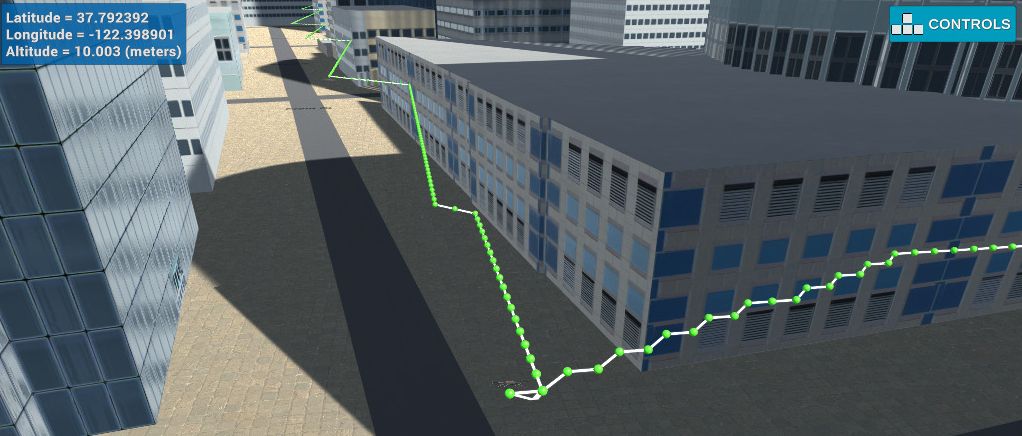
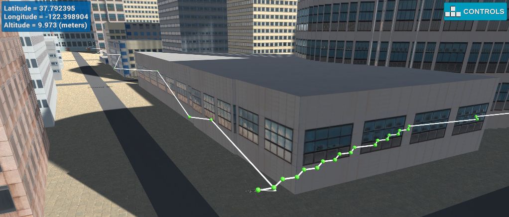
To add some additional fun, the provided CSV file conflicts with the scenery. Here's a path that leads straight through a house because that spot is indeed labeled as free according to the map, at a 10 meter altitude.
When we compare this with the height map generated by the provided colliders.csv,
we find that this building, indeed, is announced to be way smaller than it
is in the simulation:
When generating a new colliders.csv straight from the Simulator, the situation has become
noticeably better for the buildings (note that the buggy building on
the starting position is now registered, too), however details such as trees are missing.
Because we obviously will not accept a situation like this, the map loading code has been
changed to combine both the provided colliders.csv and the file generated by the simulator,
labeled as colliders.additional.csv. If you look closely, the tall building that makes for
one of the "optional" waypoints in LOCATIONS.md is appearing as an easily accessible
space in the map and because of that, the drone will crash into a building when it goes there -
but one problem at a time.
Back in the core business, the paths generated by the A* algorithm tend to exhibit either
- long sequences of identical steps, or
- extremely zig-zaggy behavior.
Specifically, the second problem occures when the required trajectory doesn't align with the available actions.
One of the simplest techniques at hand for the first of the two problems is to utilize a collinearity test for neighboring points, and so this is what was added first. However, the implemented form of a collinearity test is only working for two-dimensional motion and is only exact for integral coordinates.
The core idea is to analyze the matrix describing the vector space spanned by three two-dimensional points in
homogeneous coordinates (x, y, 1) and to determine its determinant (pun somewhat intended).
If the determinant is zero, this implies that all rows (or columns) are dependent, that is, are identical up
to a coefficient - put differently, they are linear combinations, so they lie on a line.
Given a matrix M consisting of the column vectors (x1, y1, w1), (x2, y2, w2)
and (x3, y3, w3) such that
    | x1  x2  x3 |
M = | y1  y2  y3 |
    | w1  w2  w3 |
we find that the equation for the determinant is
det(M) = x1 (y2 w3 - y3 w2) + x2 (y3 w1 - y1 w3) + x3 (y1 w2 - y2 w1)
Since we are dealing with homogeneous coordinates, the coefficients w1, w2 and w3 are all
defined to be 1, and we're left with the following Python code for 2D collinearity tests:
def are_collinear(p1: GridPosition, p2: GridPosition, p3: GridPosition) -> bool:
    det = p1[0] * (p2[1] - p3[1]) + \
          p2[0] * (p3[1] - p1[1]) + \
          p3[0] * (p1[1] - p2[1])
    return det == 0
What is left is to iteratively move through the list of points and drop every center point of
every three collinear neighbors. This is implemented in prune_waypoints_fast().
As mentioned in the previous section, another issue in the generated paths are alternating actions, creating a zig-zag or staircase pattern.
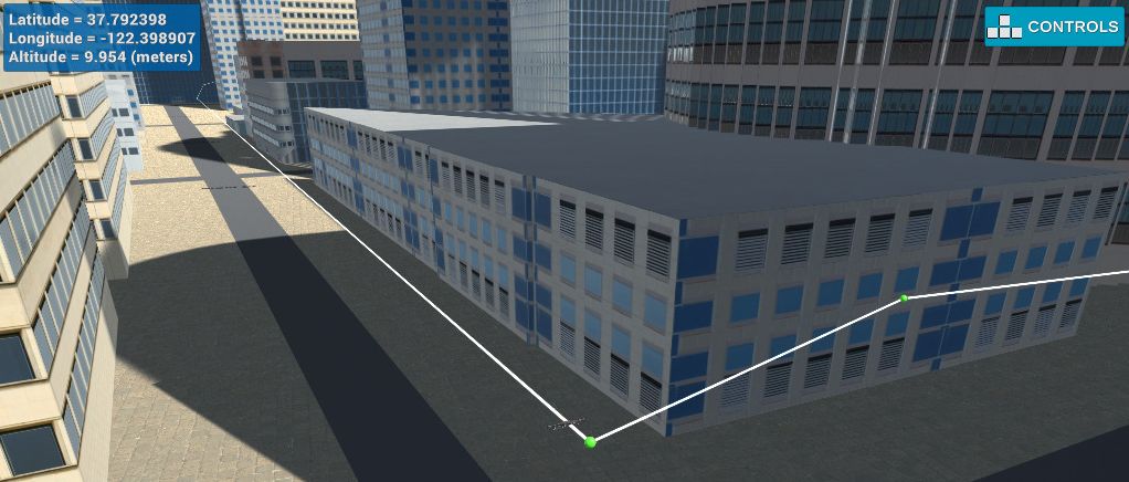
After initially cutting down on waypoints by using collinearity tests, we apply another pruning layer by means of raycasting. Here we draw a line between the current point and the point two steps ahead. If each point on this line lies in free space, we can drop the point in between (our immediate neighbor). Since we already use an integral grid, we can make use of the Bresenham line algorithm.
This technique is implemented in the prune_waypoints_raycast() and, by extension, line_test()
method in pruning_utils.py. The implementation is based on Petr Viktorin's bresenham
Python package, with a modification for grid occupancy tests.
This operation is generally somewhat more costly than the previous approach as we need to test each coordinate generated by the algorithm. However, since we already pruned the total number of waypoints using the collinearity test, this should not only be faster, but will also drastically improve the quality of the generated path.
At the end of the day, always park your drone in a safe spot (and don't forget to disarm it).
