Behavioral Cloning Project
My goals for this project are the following:
- Use the simulator to collect data of good driving behavior
- Build a convolution neural network in Keras that predicts steering angles from images
- Train and validate the model with a training and validation set
- Test that the model successfully drives around track 1 without leaving the road
- Test that the model successfully drives around track 2 being trained only on track 1 data
- Describe the process and summarize results
- Provide insight into the processes described in the model through visulizing attention
Note: the data included in this repository in the "data" folder is not the data used to train the model, it is only there for example purposes only due to the data set size
Data was gathered from the simulator provided by Udacity. After considering the lesson material, I used a few guidelines for data collection:
- Used the mouse pad rather than key arrows get more unique steering angles
- Add instances of purposefully drifting out of ideal locations and recover to lane center
- Drive backwards down the track as well as forwards
- Record repeat instances of navigating curves, begining at different locations in the lane
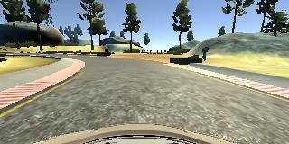
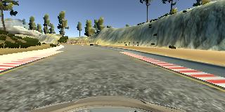
Following these guidelines, I collected 13,701 images from track 1 only in the simulator. In the below example shows a typical image colleced.
Typical dash cam training image collected with the simulator.
After collecting data, I applied 3 major preprocessing operations to resulting images:
- Doubling the data by adding a flipped (a pixel by pixel reflection over the vertical center) version of each image to the "X" or independed data and modified its corresponding steering angle by multiplying negetive one by the original angle to the "y" or dependent variable.
- Putting the doubled data set through up-and-down sampling to create a smaller data set which exibited a more uniform distribution over the steering angles.
- A more aggresive cropping operation than was suggested in the class material
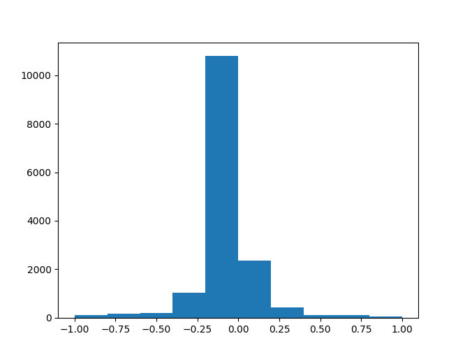
Here, the raw collected data was most often a negetive steering value close to zero. This was because the track was mostly oval and driven most often in a counter clockwise direction.
The original distribution has more negetive steering angles than positive. f
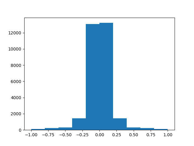
After the reflecting process, the steering angle distribtion is more balanced.
Cropping was performed along with image and steering angle reflection. The more aggressive vertical crop (taking some pixes off the top and bottom to remove extraneous views above the road and the dash board) required editing the drive.py file to be compatible with the new image size.
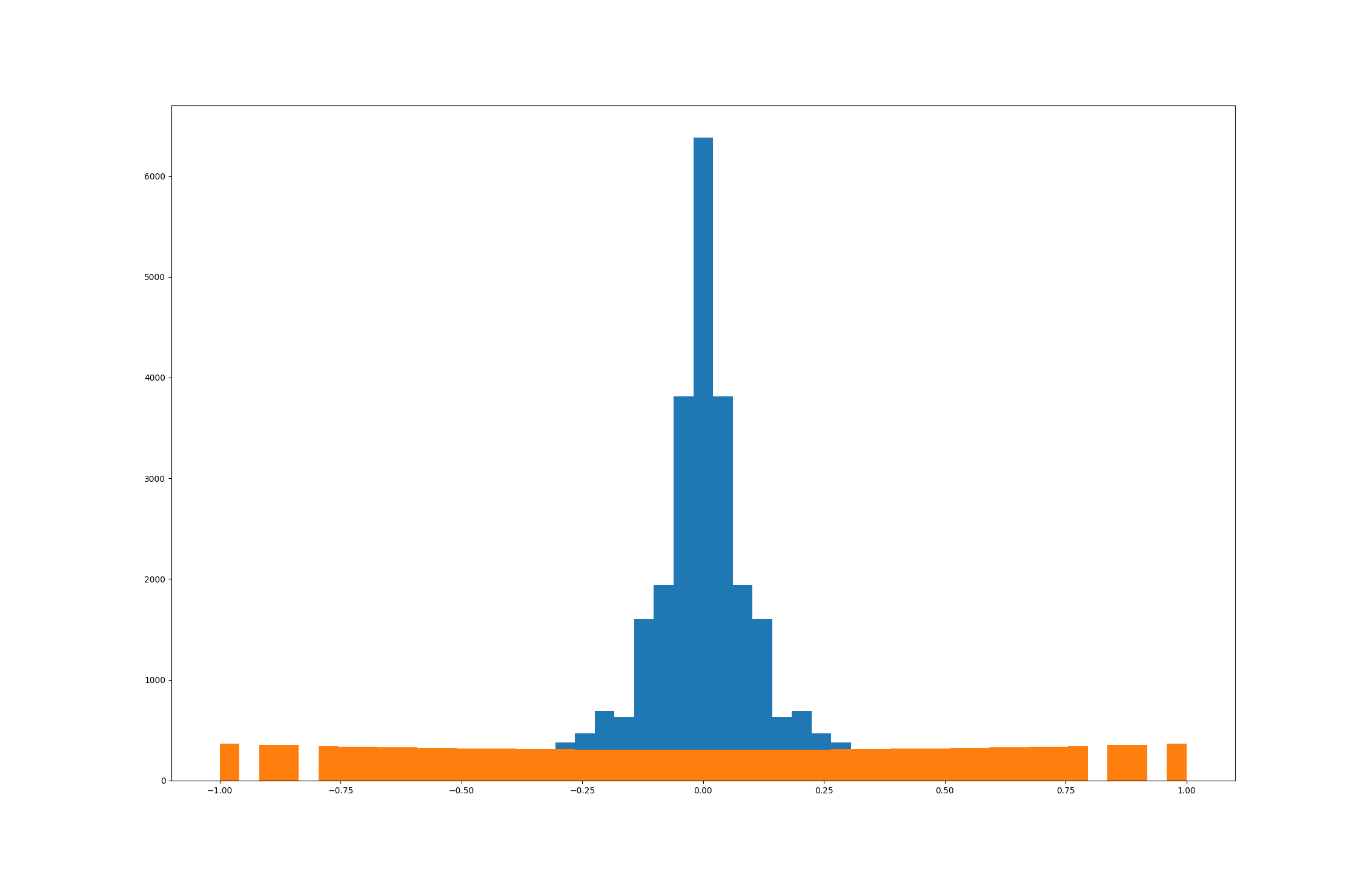
These preprocessing steps were done in preperation of building a data generator to agument the existing data, which selects a random sample of images and performs some operations on them for each training batch. Through trial and error training of different models with data sets demonstrating different dependent variable distributions (right skewed, student's t) a data set with a more uniform distribution of steering angles was preferable. I wrote a function that would down-or-up sample the total number of images and up-or-down sample images depending on their corresponding streering angle with a parameterized function based on a the shape of a parabola centered at steering angle zero and a selectable number of histogram bins. This way I could experiment with different sampling techniques and resulting dependent variable distributions. Again by trial and error, I found a 500 bin histogram with larger steering angles upsampled about 30% more than those near zero consistantly trained models that easily navigated track 1. Also, bin size ended up being extremely important, as the specific images selected to be upsampled could be very different between 10, 20, 50, or more bins. More bins meant high steering angles were more likely to be well represented, and a lower number of bins made it more likely that a wider range of images would be in the final data set. It was very important to plot the data with a various number of histogram bins to get a good feel for the variable density through the steering angles.
Steering angle distribution for preprocessed (blue) and final respampled (orange) data sets in 500 bin histogram
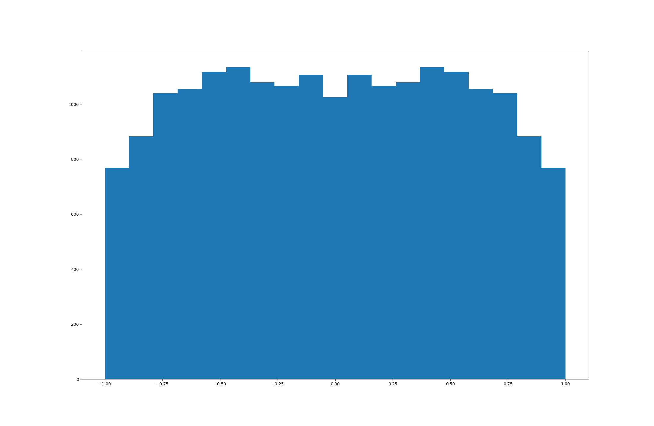
Final respampled distribution viewed with a 20 bin histogram
Interestingly, I found that a nearly perfect uniform distribution was not a great indicator of future model performance on its own, but rather, there were optimum parameters and specific choices in the sampling process that produced consistantly better models. My hypothesis is that I didn't have enough variety of very large steering angles to upsample them so much, and ended up skewing the data to a large subset of very similar images. I left this hypotheis untested in this project, and rather took away the reinformcment that careful attention to the specific data at hand is important in machine learning applications. The field of neural computing is still new enough that emerging general guidelines are secondary to specific knowledge of data sets, the problem space in which complex models are trained and applied, and trial-and-error proof of concept.
I chose to use keras image data generator to augment the data set resulting from the preprocessing steps. I used a combination of the built in options and my own functions for data augmentation. In preperation for a training / validation split, I build a separate generator for each. I ended up useding slightly different parameters for training and validation generators. For the training generator:
- Randomly rotate image up to 15 degrees
- Ranodm color channel Shift up to 35
- Custom random bright and dark spot function
For the validation generator:
- Randomly rotate image up to 20 degrees
- width_shift_range 0.05
- Ranodm color channel Shift up to 45
- Custom random bright and dark spot function
In addition to the built in options, I wrote a function which creates a random number (from 0 to 5) of randomly bright and dark spots in addtion to the built-in options in image data generator. All of the parameters where chosen by trial and error model training.
Below are a number of examples from the validation generator.
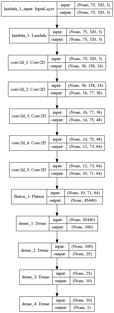
Over the course of this project I trained many different models with differnt architectures. I found that models with millions of parameters did not nessesarily perform better than models with only a few hunderd thousand. Additionaly, models with less than a million parameters more often generalized to track 1 and track 2 better. I trained the arcitecture below multple times and it performed consistantly well with different random samples of training data and different train test splits at around 10 epochs. The model presented here was trained for 20 epochs.
I started with a similar architecture to the class material, and eventually went with a model similar to Jeremy Shannon's in [https://github.com/jeremy-shannon/CarND-Behavioral-Cloning-Project]. It is worth noting that many of the different architectures I tested performed well once the data was preprocessed and augmented, however, some performed better than others and this architecture consistantly perfromed well. After testing relu, elu, tanh, and even a custom activation, I went with elu. My theory is that elu is a more symetrical function than relu, and may somehow provide better results across the regression range. I did not test this theory here in the interest of time.
Structure of Model Completing Track 1
The data was split into training and validation sets, and validation checks were performed after each training epoch. Although lower validation loss generally was evidence for a better model, this was not always the case. Sometimes, validation results seemed a poor predictor of model performance on new data. Additionally, depsite experimenting with a wide range of approaches and parameters, I rutinely saw a validation loss lower than training loss. After a while I defaulted to just testing the solution after training to a point where both losses were below 0.1 MSE. Currently, I don't have a good hypothesis for why this happened. The description below produced validation losses slightly more than training losses more often then most of my other approaches.
After some brief experimentation, I opted for the adam optimizer with a learning rate parameter of 0.0001. I saved different models at various epochs in during training to compare their attention maps later. The goal here was to have an oportunity to visualize what the network is learning and try to explain why it predicts a particular steering angle. In general, the model would start performing well at around 10 or more epochs with the learing rate set to 0.0001, and about 4 or 5 epochs when set to 0.001. However, I consistantly achieved a lower loss with a learning rate of 0.0001.
Additionally, I found samples per epoch and batch size to be very sensitive hyper parameters during training. Through trial and error, I ended up with 5000 samples per epoch and a batch size of 32. I tried samples per epoch up to 15000 and as low as 500, and batch sizes ranging between 1 to 256. For the larger numbers, there seemed to be a loose threhold of diminishing returns in terms of final loss vs training time, and for the very low numbers, the final loss was usually worse. Some middling values seemed to perform consistantly better.
Navigating track 1 successfully
Unfortunately, my solution was not able to generalize to track 2. Interestingly, I found that a model with max pooling layers usually generalized better to track 2 than a model without, although it might drive track 1 a little worse. My solution descrived here contains no max pooling layers, which consistantly navigated track 1.
Navigating track 2 to the first big turn
Spurred on by this failure to generalize to track 2, I decided to attempt a visualization of what the network was seeing to gain insight into why it failed to generalize, maybe gain some knowledge of specific weak points in the predictions, and even provide evidence of model efficacy.
We build a lot of complex models at my current job which are used to make predictions and estimations that influence policy. In this application, it is of utmost importance that we can explain and describe how the models work and why they say what they say. I'm seeing an increasing focus on interpretation in the mahcine learning world as well, and in my oppinion it will be important for practitioners, especially in the deep learning field, to be able to look into the "darkness" of complex models and provide some understaning into how they work and why cerntain predictions happen when communicating with policy makers or legal professionals.
To take my own advice, I searched for different tools and found keras-vis [https://github.com/raghakot/keras-vis]. In order to use this here, I upgraded to keras 2.0. Building off a provided example [https://github.com/raghakot/keras-vis/blob/master/applications/self_driving/visualize_attention.ipynb] I wrote a function wich would overlay an attention map on recorded images from drive.py. Attention can loosely be interpreted as which parts of the image were important for the model to make a prediction. What I want to see is clear highlighting of lane lines, similar to the finding lane lines project. In my oppinion, this would indicate a model which understands that lane line are the most important object in predicting seering angles, rather than something else like shadows or peripheral objects.
Since the behavioral cloning application is a regression of a variable with range [-1, 1] I repeated this process for large negetive steering angles (left turn), large positive steering angles (right turn), and small steering angles (maintain steering), following the referenced example. Below is an example of before and after overlaying an attention map for the small values. You can see that the lane lines are lit up, though the model is focusing on some peripheral objects. This is not a perfect view into how the network operates, but it does provide some interesting information.
Raw collected image
Image with attention overaly heat map, from low (blue) to high (red)
Below is a video of the dash cam from the car navigating the track 1 bridge and the next 2 turns with three different attention overlays. It is encuraging to see the left turn will sometimes focus heavily on the right lane line, and the right turn on the left line. The maintain straight signal seem to watch both lines most of the time. However, the attention is noisy, and at times focuses heavily on peripheral objects, which likely causes overfitting to track 1 and the inability to generalize to track 2.
My solution achived 6 of my 7 goals. It was unable to navigate track 2 with only track 1 data. I suspect that collecting data of track 2 would make it possible to train a model which navigates both tracks entirely, but I will leave that for future work. I was happy to find a way to attempt to understand and interpret the convolutional neural network through attention maps and with some effort, I found the network was really starting to see the lane lines. There were however, still instances of attenion pointed at periferal features in images, which would lead to poor generalization. Based off these results and interpretations, a second round of this project may see more success with some data collected from track 2, even more aggresive cropping, and more carefully collected data. I struggled to collect good quality data with my laptop and found driving the car well to be a very difficult task. This ended up being a large component of the project and I admittedly "called it good" after a while. If I did it again I would hire someone who is good at video games to collect my data.
Although untested in this project, I think adding some memory to the model could improve the results drastically. As it stands, the model makes free-standing predictions for every single picutre. In real life, it is rare that the next steering angle would be so independent of the previous few. Adding memory of the last few predictions could really smooth out the model and perhaps reduce some of the confusion shown in attention of the track 2 failure video. You can really see the attention jumping around in some of the videos, I suspect smoothing this out would create a better ride.
