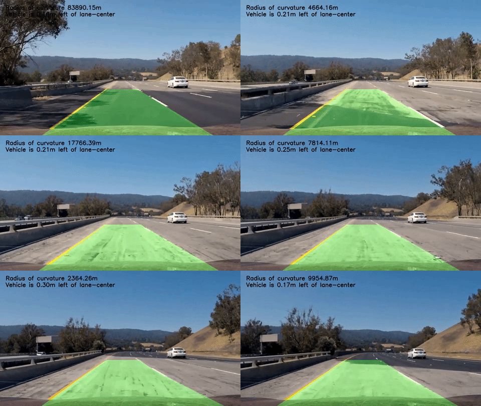
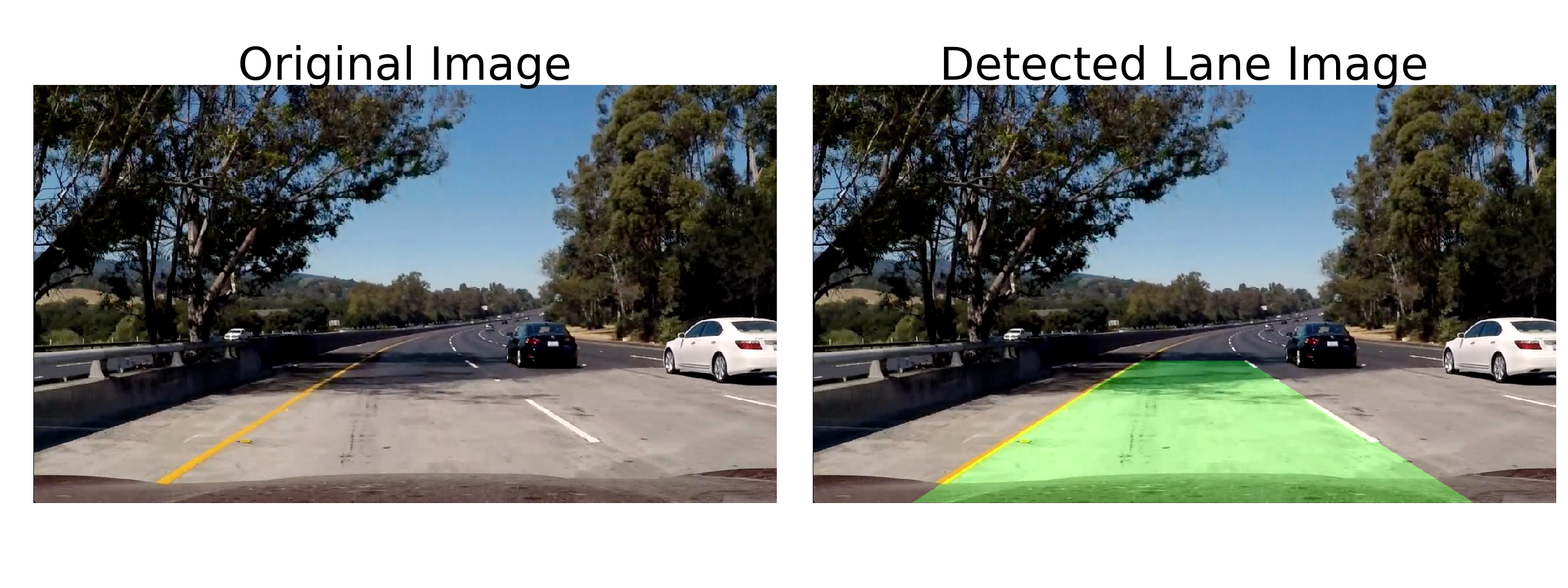
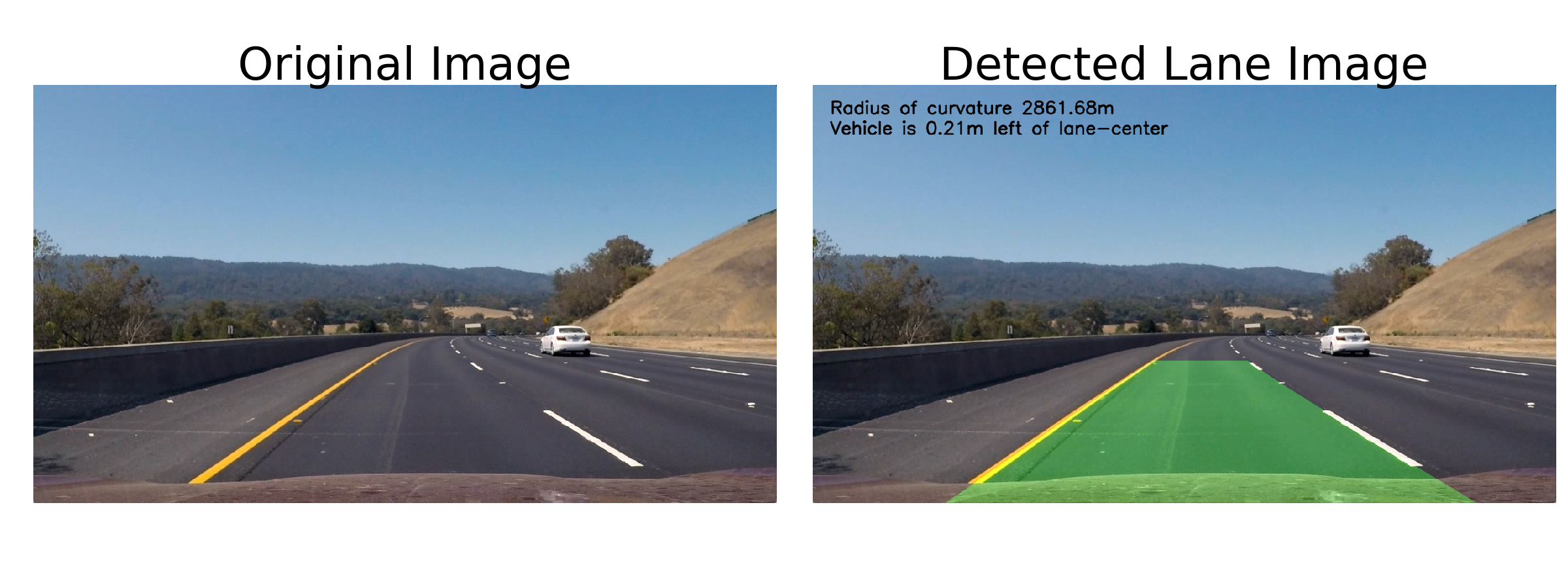
Lane detection

Lane detection on roads using camera image-feed.

Overview

This project is part of Udacity's Self-Driving Car Nanodegree program and much of the source comes from the program's lecture notes and quizzes.

Following steps were performed to achieve a lane-detection pipeline which can look for lanes in a video.

Camera calibration : Finding camera's calibration matrix and distortion coefficients.
Distortion correction : Un-distorting source images.
Image filtering : Filtering an image containing a lane based on gradient and color values of its pixels.
Image warping : Applying perspective transformation to get a "birds-eye" view of the filtered-image.
Lane detection and update : Computing polynomial fits of the lane's left and right lines.
Computing lane-curvature and vehicle offset from lane-center.
Image warping : Projecting back detected lane on top-down view of the image to the original image.
Writing the output image to an output-video.

Dependencies

Python-3.5
OpenCV-Python
Moviepy
Numpy
Matplotlib
Pickle

Running the detection routine

Switch to the source directory src:

cd src

Run the lane-detection script. This will take the video (project_video.mp4)[project_video.mp4] as its input, runs the detection pipeline on it and saves the output to detected_lane.mp4 in the parent directory.

python lane_detection.py

Directory Layout

src : Contains the following source files.

File	Description
line.py	Line class capturing the characteristics of a lane-line.
vision_util.py	Visualization and detection utility.
lane_detection.py	Contains lane-detection pipeline with other (sub)pipelines like camera-calibration and image-warping.
calibration.p	Pickled camera calibration matrix and distortion coefficients.
perspective_transform.p	Pickled perspective transform and its inverse transform matrices

camera_cal : Chessboard images for camera-calibration.
test_images : Images of lanes which we used for testing the pipeline.
output_images: Outputs from different parts of the pipeline which were applied to images in test_images.
detected_lane.mp4 : Output video containing the detected lane annotated with lane-curvature and vehicle-offset from lane-center values.

Detection pipeline description

Let's go through the detection routine steps mentioned above.

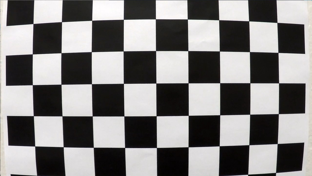
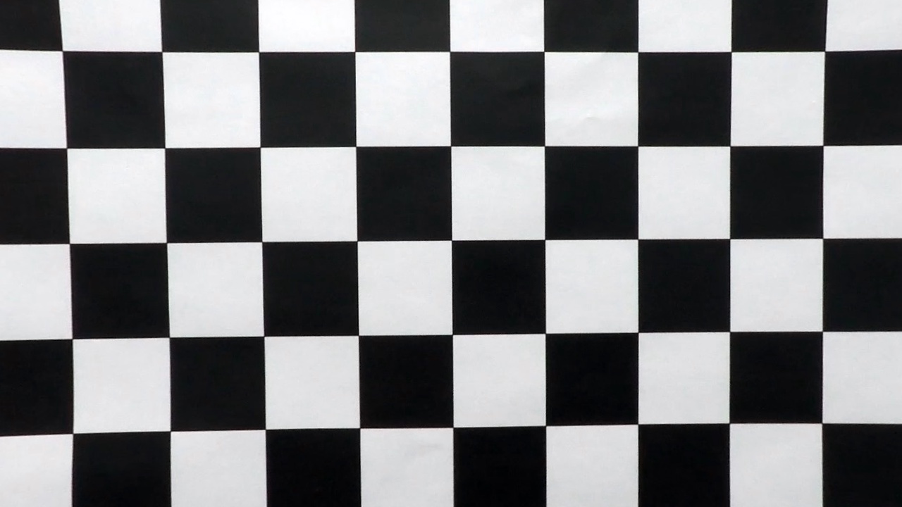
Camera calibration and Distortion correction

In this step, the camera is calibrated in order to remove its distortion effects (radial and tangential). Chessboard images in the folder camera_cal/ were used, where the following steps are taken:

Converting chessboard images to grayscale and identifying corners.
Identified corners are used to map a set of image points to points in real-world space, according to which the calibration matrix and distortion coefficients are found.
Calibration matrix and the distortion coefficients are saved in a pickle file (src/calibration.p) for reuse.

Above steps are performed in src/lane_detection.py, under calibration_pipeline() function, where OpenCV's findChessboardCorners and calibrateCamera() utilities are used.

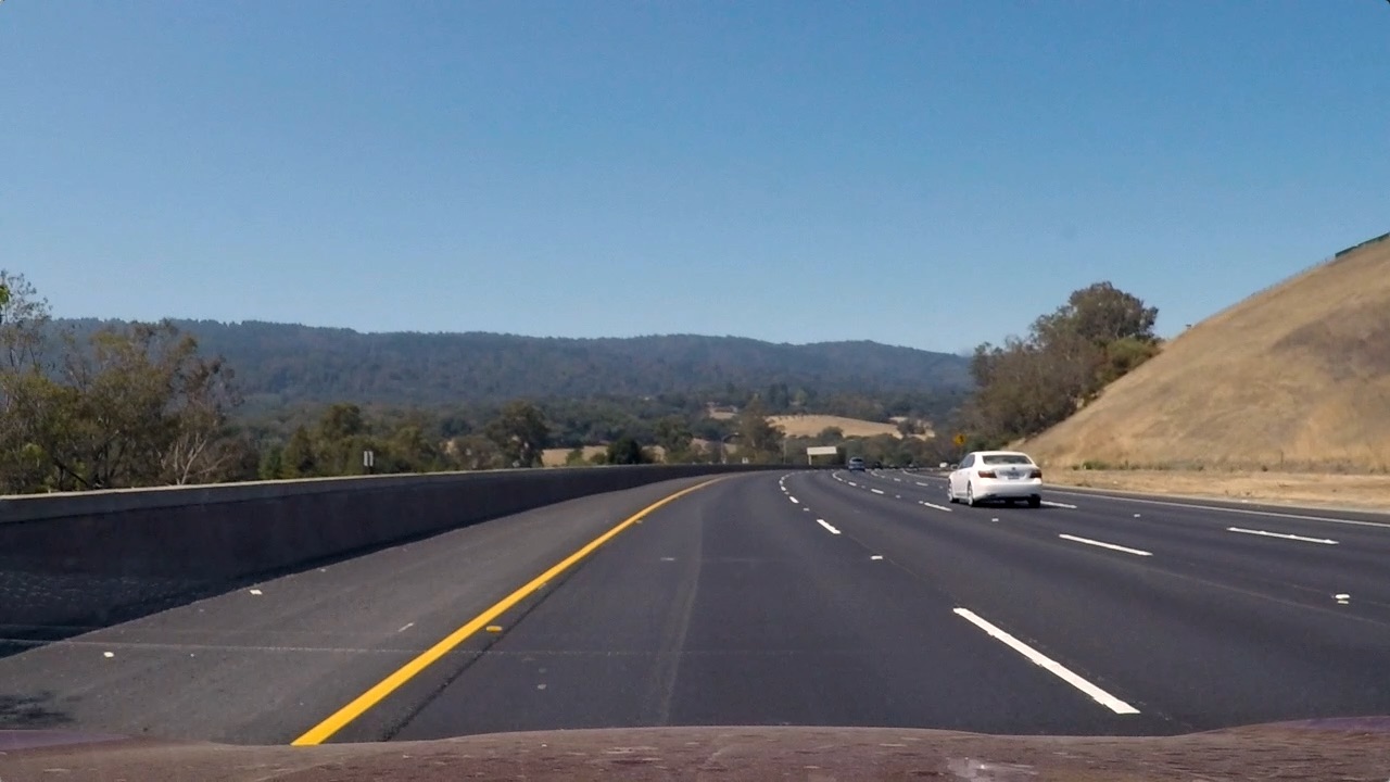
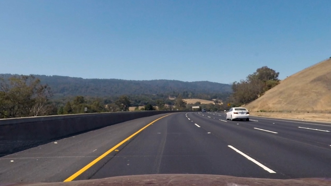
Sample (distorted) image	Undistorted version after calibration

Image filtering

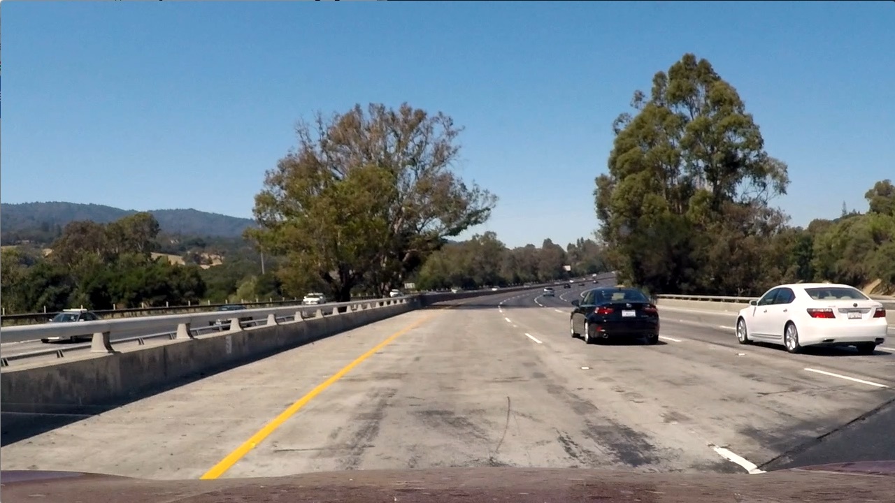
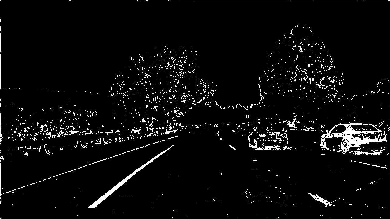
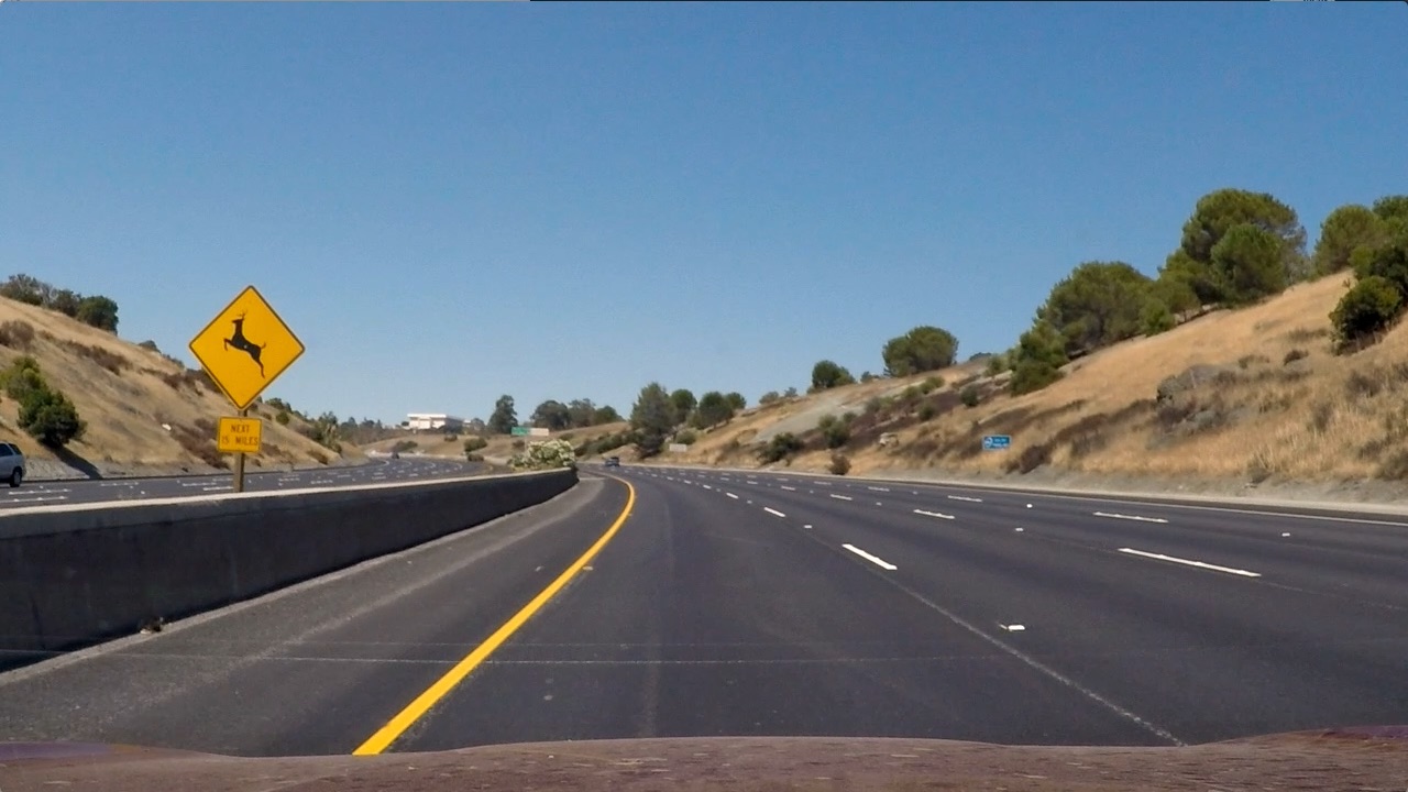
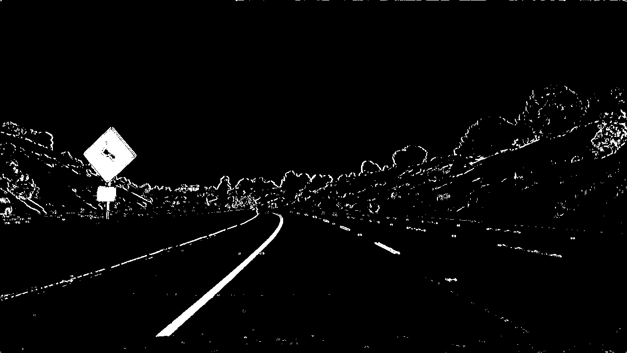
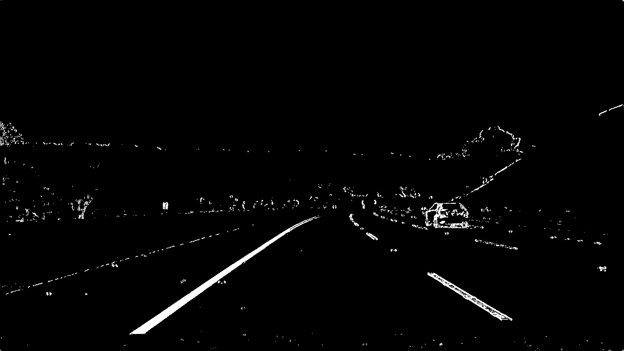
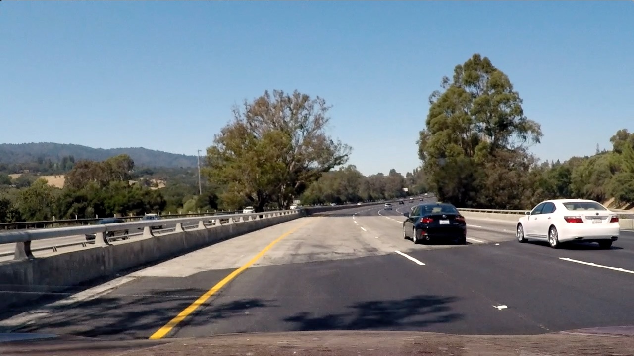
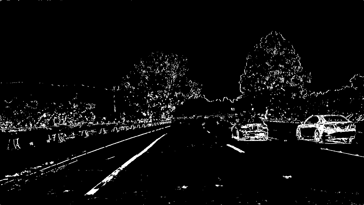
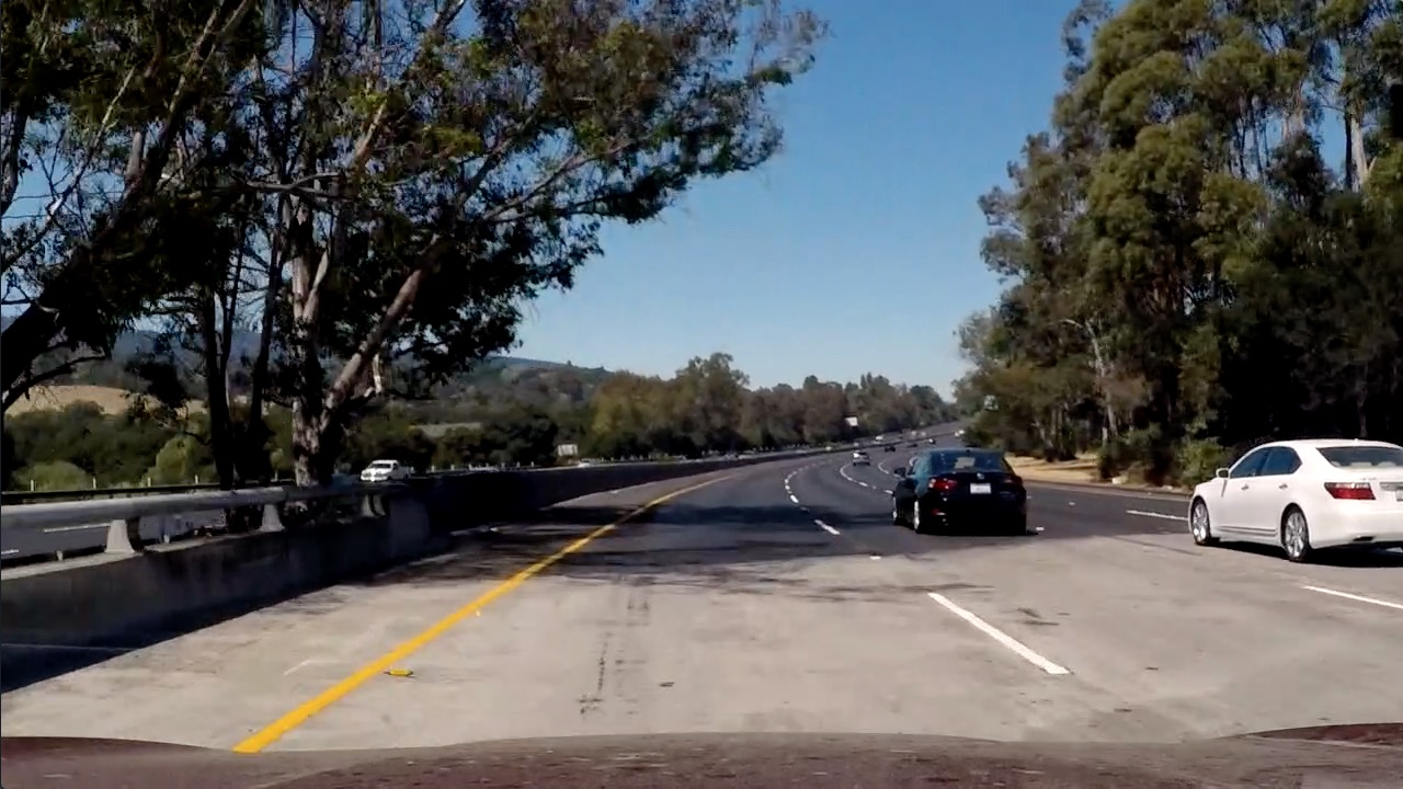
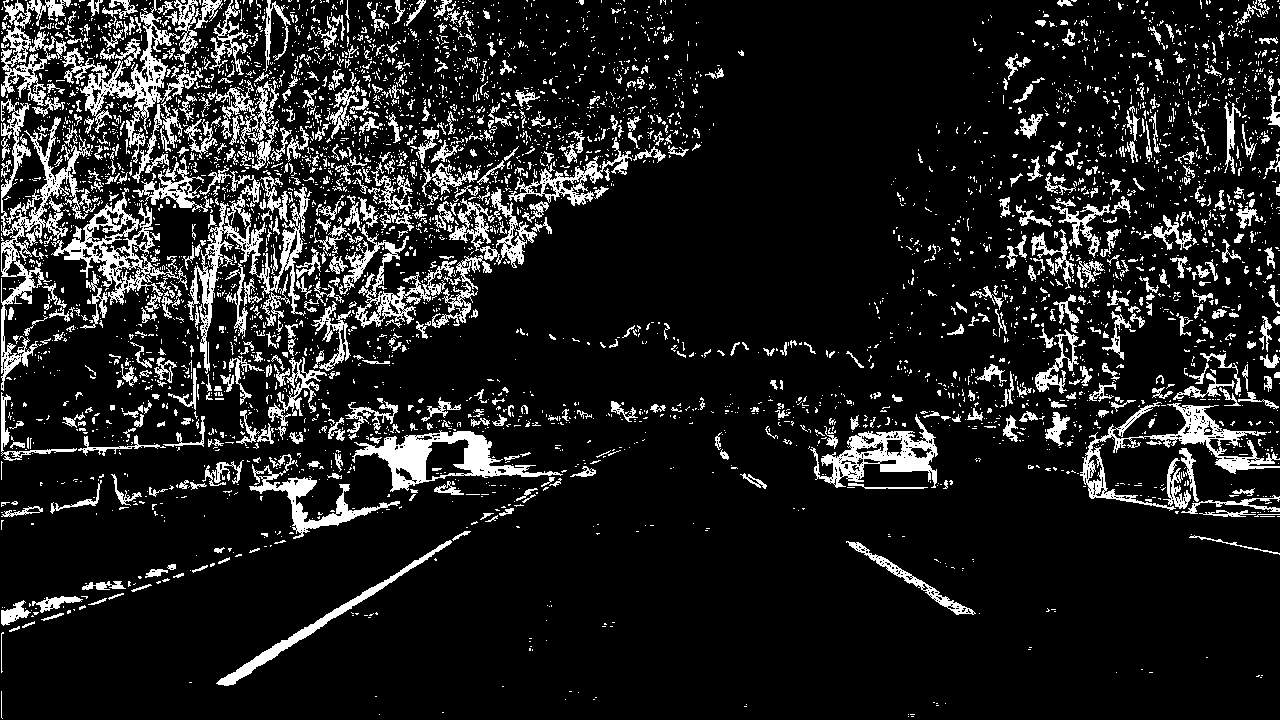
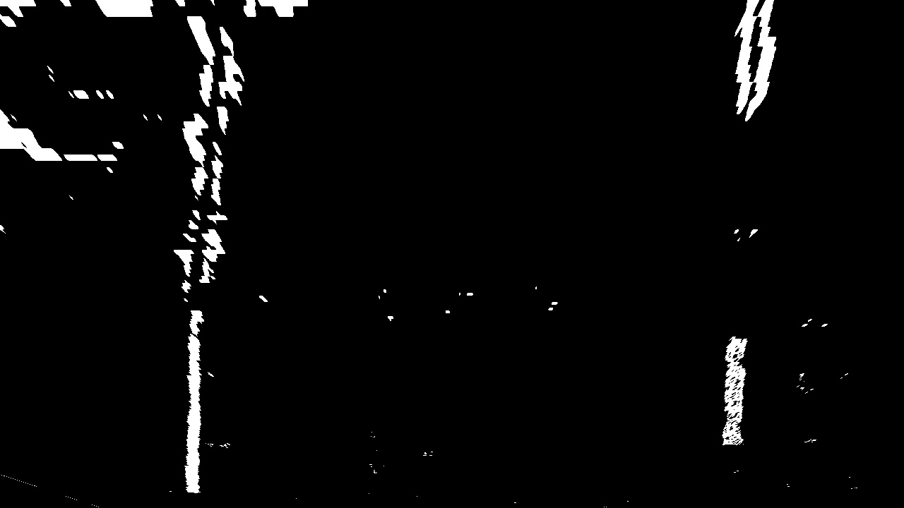
In order to identify the lane in an image, an input image (undistorted) is filtered with respect to its pixel gradients and color values, and a binary-image is returned. Following thresholds are applied.

Gradient threshold

Sobel filter on absolute value of pixels in x-axis is applied.
Sobel filter on both x and y-axis is applied and its gradients are thresholded with respect to the magnitude of scaled pixel values, scaled between 0 and 255.
Sobel filter along a given direction is applied on the gradients, targeted direction approximately sitting between π/4 and π/2.

Color threshold

Input image in RGB colorspace is converted to HLS (Hue, Light and Saturation) colorspace, where it is thresholded with respect to the Saturation channel (S-channel) values.

Above thresholding steps are carried out in combined_threshold() in src/vision_util.py. Sample binary-images for images in test_images/ directory obtained from this routine are saved in output_images/binary/ directory.

Undistorted color image	Binary image after image-filtering

Image warping for bird's eye view

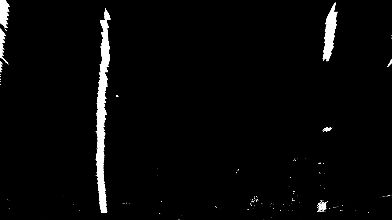
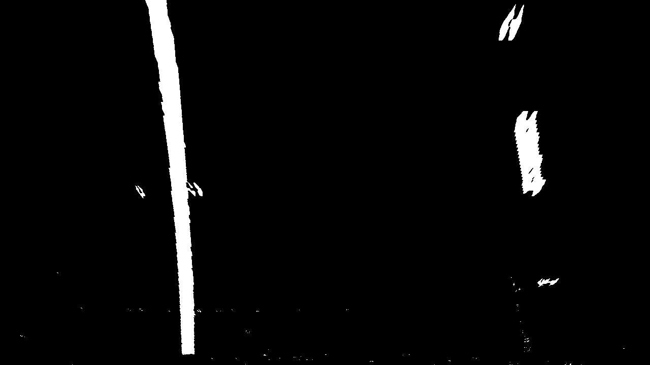
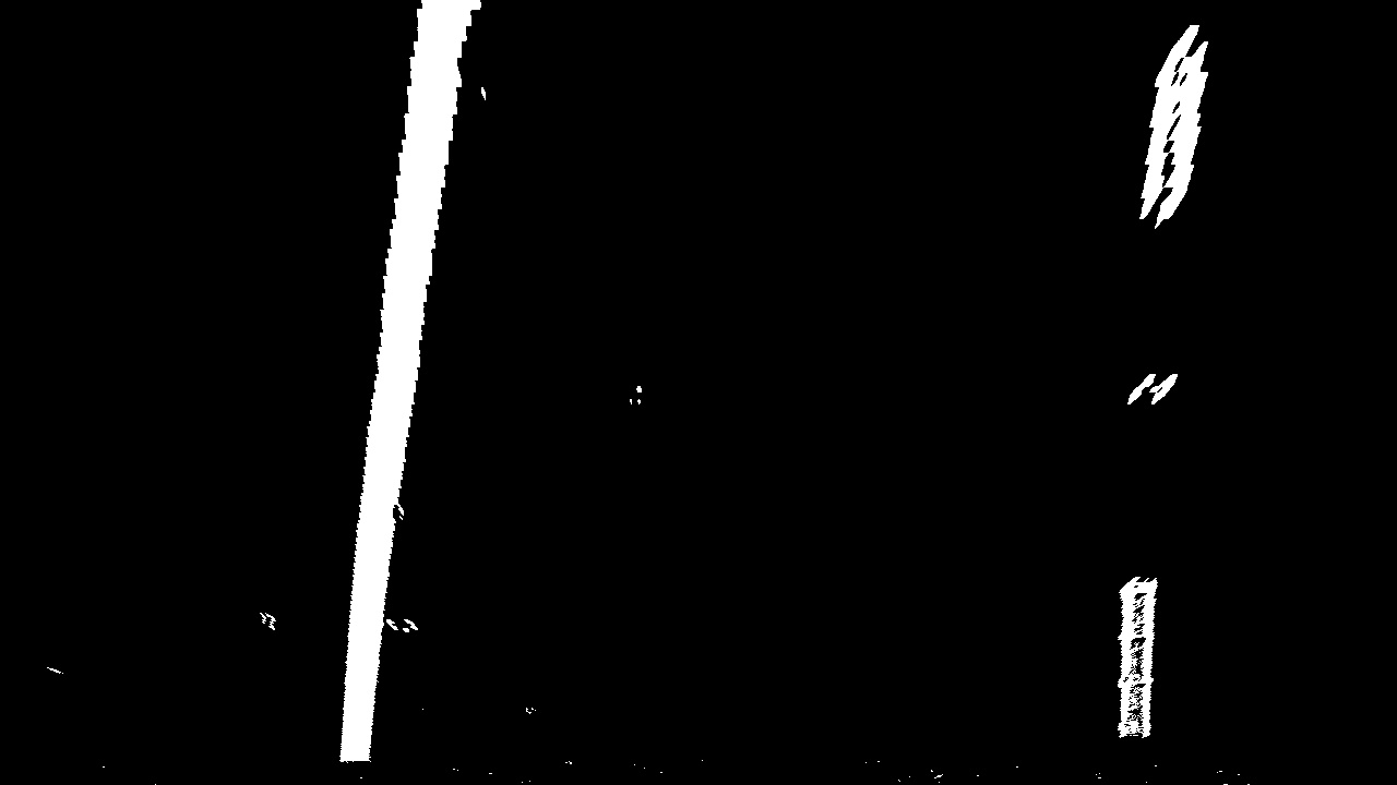
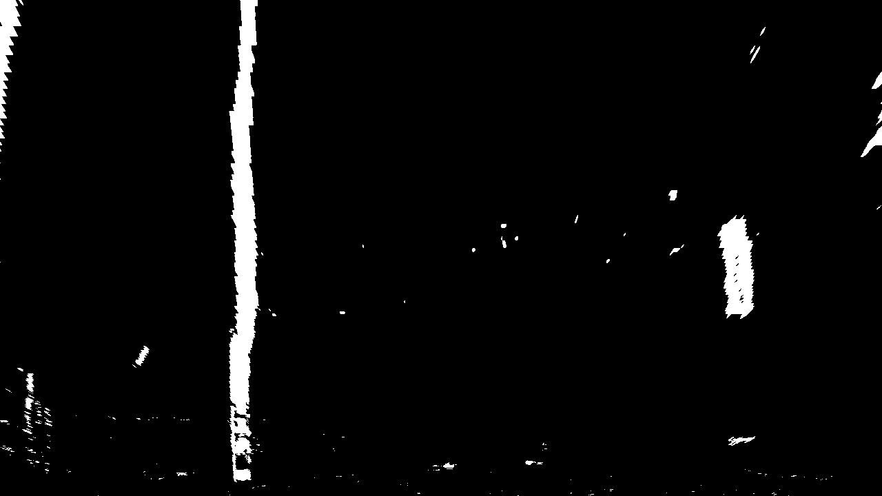
Binary image obtained from the above routine is warped to get a bird's eye view on the lane, with which we can identify lane-lines and fit polynomials. Perspective transformation is applied on the input image using OpenCV's getPerspectiveTransform(..). Steps that this routine captures:

A (hardcoded) region of interest (ROI), in form of a 4-sided polygon, in the source binary image is selected.
ROI's four vertices are projected to rectangular coordinates with a random offset (set to 100 pixels) in x-values of the pixels. This projection/mapping gives us the perspective transformation matrix.
This transformation matrix is saved in a pickle file (src/perspective_transform.p) for reuse.

Above steps are available in vision_util.py under find_perspective_transform() function. Future use of the matrix involves calling OpenCV's warpPerspective(..) function to warp the image. Sample warped binary images having bird's eye view of the lane are stored in output_images/binary_warped.

Filtered binary image	Warped binary image having bird's eye view

Lane detection and update

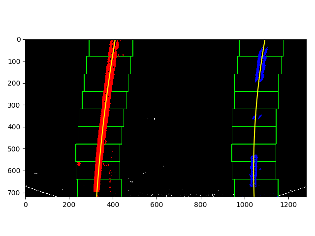
Once we have the warped binary image, we look for lane-lines doing the following:

Histogram of pixel intensities is found to find the starting x-indices of left and right lane-lanes at the bottom part of the image.
By iterating through the image bottom-up through multiple windows, and by making use of the starting indices obtained from the above step, left and right lane-lines' pixel indices are found in the +/- 100 pixel-margin around the previous windows' detections. Windows' centres belonging to left and right lane- lines are adjusted in each iteration to represent the mean of their respective detected-pixels' indices.
After collecting the lines' pixel indices, a second-order polynomial fit is performed which gives us the equation of the lane-lines.

Above steps are performed in src/vision_util, detect_lane_lines() function.

Subsequent detections make use of the polynomial equations found above:

To do a targeted search in the region around the lane-lines' curve where there's a high chance of finding/extending the lane-lines. This is carried out via a lane-line-update routine, as present in update_detected_lane() function in src/vision_util.py.
In addition to doing a targeted search, lane-lines' are smoothened by performing a moving-average on their polynomial coefficients. This is done in src/line.py's update_fit() function, which makes use of eight image-frames (utmost) to cache and average the coefficients.

Sample warped binary image	Polynomial fit on lane-lines

Lane curvature and vehicle-offset

Polynomial fits on lane-lines are made use of to compute the lane's radius curvature and the vehicle's offset's from the lane-center. We make use of (known) scaling factor which maps image resolution to metres in the world-space i.e. 3.6 metres per pixel in x-dimension and 30 metres per pixel in y-dimension.

calculate_curvature() in src/vision_util.py computes the curvature of the lane as per the second-order differential equation mentioned here.
calculate_vehicle_offset() in the same file computes the offset from finding the difference between the lane-line's center and the image's center.

Annotated source image with detected lanes

Once we find the lane-lines, we project back the lane-annotated version of the image back to the original image as shown below. This is done via doing an inverse perspective transform that we did earlier while warping for bird's-eye view of the image.

Further we annotate the original image with the curvature and vehicle-offset details. All these steps are carried out in draw_lane() function under src/vision_util.py.

Finally, the above pipeline steps, except for camera-calibration are put together in lane_detection_pipeline() function in src/lane_detection.py. This function is run against an input stream of video project_video.mp4, and the output is saved in detected_lane.mp4.

Further improvements

There are various scenarios where this lane-detection pipeline would fail for example in cases where there's occlusion (from other vehicles), where there are continuous streak of shadows with lower visibility, etc. This drawback was observed in the challenge-videos of the project.
Detection routine above is reliant on ROI to begin with. It'd make the pipeline more robust if we look for pixel features representing lane-lines rather than looking for lane-line pixels in an ROI. Making use of convolutional neural nets as outlined in works like this would improve the robustness of the detection-pipeline.

ashishraste / CarND-AdvancedLaneDetection