Advanced Lane Finding Project
The goals / steps of this project are the following:
- Compute the camera calibration matrix and distortion coefficients given a set of chessboard images.
- Apply a distortion correction to raw images.
- Use color transforms, gradients, etc., to create a thresholded binary image.
- Apply a perspective transform to rectify binary image ("birds-eye view").
- Detect lane pixels and fit to find the lane boundary.
- Determine the curvature of the lane and vehicle position with respect to center.
- Warp the detected lane boundaries back onto the original image.
- Output visual display of the lane boundaries and numerical estimation of lane curvature and vehicle position.
1. Briefly state how you computed the camera matrix and distortion coefficients. Provide an example of a distortion corrected calibration image.
The code for this step is contained in the IPython notebook located in "./camera_calibration.ipynb".
I start by preparing "object points", which will be the (x, y, z) coordinates of the chessboard corners in the world. Here I am assuming the chessboard is fixed on the (x, y) plane at z=0, such that the object points are the same for each calibration image. Thus, objp is just a replicated array of coordinates, and objpoints will be appended with a copy of it every time I successfully detect all chessboard corners in a test image. imgpoints will be appended with the (x, y) pixel position of each of the corners in the image plane with each successful chessboard detection.
I then used the output objpoints and imgpoints to compute the camera calibration and distortion coefficients using the cv2.calibrateCamera() function. I applied this distortion correction to the test image using the cv2.undistort() function and obtained this result:
Implementation of pipeline can be found in Advanced_Lane_Line_Finding.ipynb notebook. Steps from this pipeline are labeled with titles in the notebook.
Distortion correction that was calculated via camera calibration has to be correctly applied to each image. It uses cv2.undistort() with loaded camera matrix and distortion coeffs parameters.
We can combine two types off thresholds: color and gradient. Gradient threshold can be obtained by running Sobel kernel over the image and finding gradients. There are 3 types of gradients that we explored: individual X and Y, magnitude and direction of the gradient. Result can be seen in image below.
I've also applied binary mask on S channel after converting the image from RGB to HSL color space. I've used S channel since it works well on both yellow and white lines. On a image below is result of only s channel extracted and after applying threhsolds.
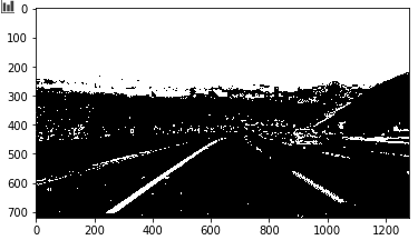
I used a combination of color and gradient thresholds to generate a binary image seen below. I used following masking: s_channel | x_sobel | (magnitude & direction).
The code for my perspective transform includes a function called perspective_transform(), which appears in the 3rd code cell of the IPython notebook. The perspective_transform() function takes as inputs an image (img), as well as source (src) and destination (dst) points. I chose the hardcode the source and destination points in the following manner:
cols, rows = combined.shape[::-1]
top_limit = np.int(rows * 0.635)
down_limit = rows - 20
src_point1 = [280, down_limit]
src_point2 = [595, top_limit]
src_point3 = [725, top_limit]
src_point4 = [1125, down_limit]
src = np.float32([src_point1, src_point2, src_point3, src_point4])

dst_point1 = [250, rows]
dst_point2 = [250, 0]
dst_point3 = [1200, 0]
dst_point4 = [1000, rows]
dst = np.float32([dst_point1, dst_point2, dst_point3, dst_point4])
This resulted in the following source and destination points:
| Source | Destination |
|---|---|
| 280, 700 | 200, 0 |
| 590, 457 | 200, 720 |
| 725, 457 | 1200, 720 |
| 1125, 700 | 1000, 0 |
I verified that my perspective transform was working as expected by drawing undistorted and warped image side by side.
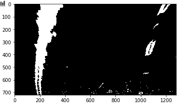
Also this perspective warp is applied on thresholded image which looks like in exmaple below.
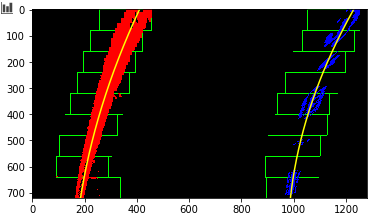
Then I did some other stuff and fit my lane lines with a 2nd order polynomial like this:
- Find histogram of pixels at the bottom half of the image as the lines are mostly vertical in that part
- Find centers of left and right lanes based on the value of the histograms for that points
- Create rectangles with lane centers and find nonzero pixels with -/+ margin from the center
- Append these pixels into left and right lane list
- If there are more pixels then given threshold we need to take this into account and calculate new center position of the next verctical rectangle. Position is calucalted as mean of given pixels.
- Now perform steps 3 - 5 for all rectangles. Number of them is a parameter and it also depends on the height of the image.
- After we have a list of pixels that should be taken into account we need to perform
cv2.polyfit()for second order polynom on those lines and get left and riht lane coefficients.
Result is seen in image below
This involves measuring how long and wide the section of lane is that we're projecting in our warped image. We could do this in detail by measuring out the physical lane in the field of view of the camera, but for this project, you can assume that if you're projecting a section of lane similar to the images above, the lane is about 30 meters long and 3.7 meters wide. Or, if you prefer to derive a conversion from pixel space to world space in your own images, compare your images with U.S. regulations that require a minimum lane width of 12 feet or 3.7 meters, and the dashed lane lines are 10 feet or 3 meters long each.
Let's say that our camera image has 720 relevant pixels in the y-dimension (remember, our image is perspective-transformed!), and we'll say roughly 700 relevant pixels in the x-dimension (our example of fake generated data above used from 200 pixels on the left to 900 on the right, or 700). Therefore, to convert from pixels to real-world meter measurements, we can use:
Define conversions in x and y from pixels space to meters: ym_per_pix = 30/720 # meters per pixel in y dimension xm_per_pix = 3.7/700 # meters per pixel in x dimension
I calculated curvature with known formula given here and following code:
curve_radius = ((1 + (2*lane_coeff[0]*y_eval*ym_per_pix + lane_coeff[1])**2)**1.5) / np.absolute(2*lane_coeff[0])
lane_coeffs are coffiecents for lane obtained after using polyfit.
y_eval is the single point for which we will do the calculs of curve
You can assume the camera is mounted at the center of the car, such that the lane center is the midpoint at the bottom of the image between the two lines you've detected. The offset of the lane center from the center of the image (converted from pixels to meters) is your distance from the center of the lane.
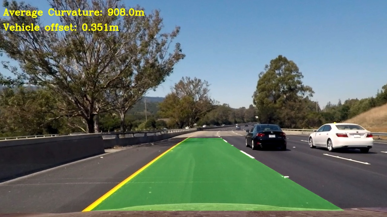
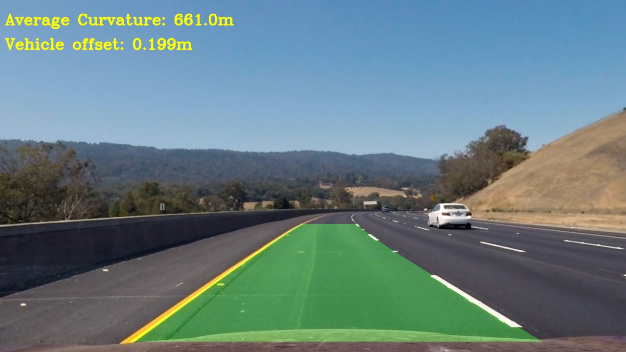
I implemented this step in lines # through # in my code in yet_another_file.py in the pipeline function PorcessLane(). Here is an example of my result on a test image:
I've run the algorithm against provided video and here's the link to my video result.
I used basic techniques of different types to obtain the resulted image. Used camera calibration, perspective transforms, different color spaces, thresholding, histograms, polynomial functions and othe.
I've used most basic approach, so there are still a lot of room to improve. Using low-pass filter, scaning ahead based on currnt line position instead of finding rectangles every time. This would speed up the processing. More playing with threshold can be done and region of interests.
There are some artifacts when vehicle encounters shadows, road damage or poor lane quality. This is understandable and expected with this approach. On more challenging videos we need to take a lot more things into aaccount like sharp turns, covered lanes (e.g. leaves), traffic infront, reflection etc.
