Compute the Euclidean Distance Transform of a 1d, 2d, or 3d labeled image containing multiple labels in a single pass with support for anisotropic dimensions. Curious what the output looks like? Download the movie!
import edt
import numpy as np

# e.g. 6nm x 6nm x 30nm for the S1 dataset by Kasthuri et al., 2014
labels = np.ones(shape=(512, 512, 512), dtype=np.uint32, order='F')
dt = edt.edt(
  labels, anisotropy=(6, 6, 30),
  black_border=True, order='F',
  parallel=4 # number of threads, <= 0 sets to num cpu
)
# see more features below- Compute the distance transform of a volume containing multiple labels simultaneously and then query it using a fast masking operator.
- Convert the multi-label volume into a binary image (i.e. a single label) using a masking operator and compute the ordinary distance transform.
pip install edtBinaries are available for some platforms. If your platform is not supported, pip will attempt to install from source, in which case follow the instructions below.
Requires a C++ compiler.
sudo apt-get install g++ python3-dev
pip install numpy
pip install edt --no-binary :all:Consult help(edt) after importing. The edt module contains: edt and edtsq which compute the euclidean and squared euclidean distance respectively. Both functions select dimension based on the shape of the numpy array fed to them. 1D, 2D, and 3D volumes are supported. 1D processing is extremely fast. Numpy boolean arrays are handled specially for faster processing.
If for some reason you'd like to use a specific 'D' function, edt1d, edt1dsq, edt2d, edt2dsq, edt3d, and edt3dsq are available.
The three optional parameters are anisotropy, black_border, and order. Anisotropy is used to correct for distortions in voxel space, e.g. if X and Y were acquired with a microscope, but the Z axis was cut more corsely.
black_border allows you to specify that the edges of the image should be considered in computing pixel distances (it's also slightly faster).
order allows the programmer to determine how the underlying array should be interpreted. 'C' (C-order, XYZ, row-major) and 'F' (Fortran-order, ZYX, column major) are supported. 'C' order is the default.
import edt
import numpy as np

# e.g. 6nm x 6nm x 30nm for the S1 dataset by Kasthuri et al., 2014
labels = np.ones(shape=(512, 512, 512), dtype=np.uint32, order='F')
dt = edt.edt(
  labels, anisotropy=(6, 6, 30),
  black_border=True, order='F',
  parallel=1 # number of threads, <= 0 sets to num cpu
)
# signed distance function (0 is considered background)
sdf = edt.sdf(...) # same arguments as edt

# You can extract individual components of the distance transform
# in sequence rapidly using this technique. A random image may be slow
# as this uses "runs" of voxels to address only parts of the image at a time.
# in_place=True may be faster and more memory efficient, but is read-only.
for label, image in edt.each(labels, dt, in_place=True):
  process(image) # stand in for whatever you'd like to do

# There is also a voxel_graph argument that can be used for dealing
# with shapes that loop around to touch themselves. This works by
# using a voxel connectivity graph represented as a image of bitfields
# that describe the permissible directions of travel at each voxel.
# Voxels with an impermissible direction are treated as eroded
# by 0.5 in that direction instead of being 1 unit from black.
# WARNING: This is an experimental feature and uses 8x+ memory.
graph = np.zeros(labels.shape, dtype=np.uint8)
graph |= 0b00111111 # all 6 directions permissible (-z +z -y +y -x +x)
graph[122,334,312] &= 0b11111110 # +x isn't allowed at this location
graph[123,334,312] &= 0b11111101 # -x isn't allowed at this location
dt = edt.edt(
  labels, anisotropy=(6, 6, 30),
  black_border=True, order='F',
  parallel=1, # number of threads, <= 0 sets to num cpu
  voxel_graph=graph,
)
Note on Memory Usage: Make sure the input array to edt is contiguous memory or it will make a copy. You can determine if this is the case with print(data.flags).
Include the edt.hpp header which includes the implementation in namespace edt. You'll need to also include threadpool.h and add the -pthread compiler flag. The code is written to the C++11 standard.
#include "edt.hpp"

int main () {

    int* labels = new int[3*3*3]();

    int sx = 3, sy = 3, sz = 3;
    float wx = 6, wy = 6, wz = 30; // anisotropy

    float* dt = edt::edt<int>(labels, sx, sy, sz, wx, wy, wz);

    return 0;
}
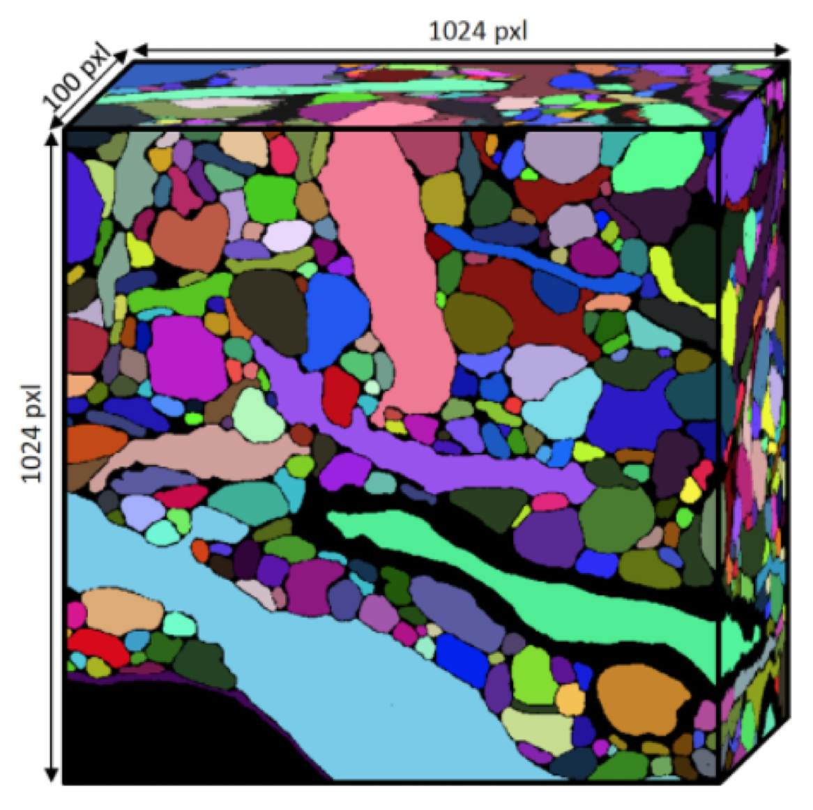
Fig. 1. A labeled 3D connectomics volume. Credit: Kisuk Lee
The connectomics field commonly generates very large densely labeled volumes of neural tissue. Some algorithms, such as the TEASAR skeletonization algorithm [1] and its descendant [2] require the computation of a 3D Euclidean Distance Transform (EDT). We found that the scipy implementation of the distance transform (based on the Voronoi method of Maurer et al. [3]) was too slow for our needs despite being relatively speedy.
The scipy EDT took about 20 seconds to compute the transform of a 512x512x512 voxel binary image. Unfortunately, there are typically more than 300 distinct labels within a volume, requiring the serial application of the EDT. While cropping to the ROI does help, many ROIs are diagonally oriented and span the volume, requiring a full EDT. I found that in our numpy/scipy based implementation of TEASAR, EDT was taking approximately a quarter of the time on its own. The amount of time the algorithm spent per a block was estimated to be multiple hours per a core.
It's possible to compute the EDT much more quickly by computing the distance transform for all labels in one pass by making it boundary aware. Since the distance transform does not result in overlapping boundaries, it is trivial to then extract individual ROIs by to querying the block with the shapes of individual labels.
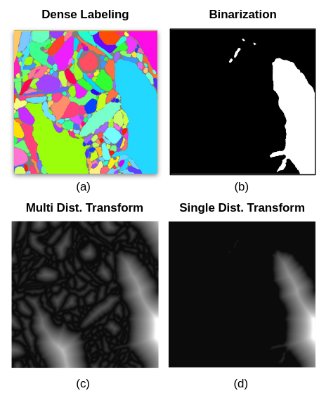
Fig. 2. Extracting the distance transform of a single label from dense segmentation. (a) a 2d slice of dense segmentation (b) extraction of a single label into a binary image (c) simultaneous distance transform of all labels in (a) (d) distance transform of (b) which can be achieved by direct distance transform of (b) or by the multiplication of (b) with (c).
The implementation presented here uses concepts from the 1994 paper by T. Saito and J. Toriwaki [4] and uses a linear sweeping method inspired by the 1966 method of Rosenfeld and Pfaltz [4] and of Mejister et al [7] with that of Mejister et al's and Felzenszwald and Huttenlocher's 2012 [6] two pass linear time parabolic minmal envelope method. I later learned that this method was discovered as early as 1992 by Rein van den Boomgaard in his thesis. [10] I incorporate a few minor modifications to the algorithms to remove the necessity of a black border. My own contribution here is the modification of both the linear sweep and linear parabolic methods to account for multiple label boundaries.
This implementation was able to compute the distance transform of a binary image in 7-8 seconds. When adding in the multiple boundary modification, this rose to 9 seconds. Incorporating the cost of querying the distance transformed block with masking operators, the time for all operators rose to about 90 seconds, well short of the over an hour required to compute 300 passes.
A naive implementation of the distance transform is very expensive as it would require a search that is O(N2) in the number of voxels. In 1994, Saito and Toriwaki (ST) showed how to decompose this search into passes along x, y, and z linear in the number of voxels. After the X-axis EDT is computed, the Y-axis EDT can be computed on top of it by finding the minimum x2 + y2 for each voxel within each column. You can extend this argument to N dimensions. The pertient issue is then finding the minima efficiently without having to scan each column a quadratic number of times.
Felzenszwalb and Huttenlocher (FH) [6] and others have described taking advantage of the geometric interpretation of the distance function, as a parabola. Using ST's decomposition of the EDT into three passes, each broken up by row, the problem becomes one dimensional. FH described computing each pass on each row by finding the minimal envelope of the space created by the parabolas that project from the vertices located at (i, f(i)) for a one dimensional image f.
This method works by first scanning the row and finding a set of parabolas that constitue the lower envelope. Simultaneously during this linear scan, it computes the abscissa of the nearest parabola to the left and thereby defines the effective domain of each vertex. This linear reading scan is followed by a linear writing scan that records the height of the envelope at each voxel.
This method is linear and relatively fast, but there's another trick we can do to speed things up. The first transformation is special as we have to change the binary image f into a floating point representation. FH recommended using an indicator function that records zeros for out of set and infinities for within set voxels on the first pass. However, this is somewhat cumbersome to reason about and requires an additional remapping of the image.
The original Rosenfeld and Pfaltz (RP) paper [5] demonstrated a remarkably simple two pass sweeping algorithm for computing the manhattan distance (L1 norm, visualized here). On the first pass, the L1 and the L2 norm agree as only a single dimension is involved. Using very simple operators and sweeping forward we can compute the increasing distance of a voxel from its leftmost bound. We can then reconcile the errors in a backward pass that computes the minimum of the results of the first pass and the distance from the right boundary. Mejister, Roerdink, and Hesselink (MRH) [7] described a similar technique for use with binary images within the framework set by ST.
In all, we manage to achieve an EDT in six scans of an image in three directions. The use of the RP and MRH inspired method for the first transformation saves about 30% of the time as it appears to use a single digit percentage of the CPU time. In the second and third passes, due to the read and write sequence of FH's method, we can read and write to the same block of memory, increasing cache coherence and reducing memory usage.
The forward sweep looks like:
f(a_i) = 0               ; a_i = 0
       = a_i + 1         ; a_i = 1, i > 0
       = inf             ; a_i = 1, i = 0
I modify this to include consideration of multi-labels as follows:
let a_i be the EDT value at i
let l_i be the label at i (seperate 1:1 corresponding image)
let w be the anisotropy value

f(a_i, l_i) = 0          ; l_i = 0
f(a_i, l_i) = a_i + w    ; l_i = l_i-1, l_i != 0

f(a_i, l_i) = w          ; l_i != l_i-1, l_i != 0
  f(a_i-1, l_i-1) = w    ; l_i-1 != 0
  f(a_i-1, l_i-1) = 0    ; l_i-1 = 0
The backwards pass is unchanged:
from n-2 to 1:
    f(a_i) = min(a_i, a_i+1 + 1)
from 0 to n-1:
    f(a_i) = f(a_i)^2
A small update to the parabolic intercept equation is necessary to properly support anisotropic dimensions. The original equation appears on page 419 of their paper (reproduced here):
s = ((f(r) + r^2) - (f(q) + q^2)) / 2(r - q)

Where given parabola on an XY plane:
s:    x-coord of the intercept between two parabolas
r:    x-coord of the first parabola's vertex
f(r): y-coord of the first parabola's vertex
q:    x-coord of the second parabola's vertex
f(q): y-coord of the second parabola's vertex
However, this equation doesn't work with non-unitary anisotropy. The derivation of the proper equation follows.
1. Let w = the anisotropic weight
2. (ws - wq)^2 + f(q) = (ws - wr)^2 + f(r)
3. w^2(s - q)^2 + f(q) = w^2(s - r)^2 # w^2 can be pulled out after expansion
4. w^2( (s-q)^2 - (s-r)^2 ) = f(r) - f(q)
5. w^2( s^2 - 2sq + q^2 - s^2 + 2sr - r^2 ) = f(r) - f(q)
6. w^2( 2sr - 2sq + q^2 - r^2 ) = f(r) - f(q)
7. 2sw^2(r-q) + w^2(q^2 - r^2) = f(r) - f(q)
8. 2sw^2(r-q) = f(r) - f(q) - w^2(q^2 - r^2)

=> s = (w^2(r^2 - q^2) + f(r) - f(q)) / 2w^2(r-q)
As the computation of s is one of the most expensive lines in the algorithm, two multiplications can be saved by factoring w2 (r2 - q2) into w2 (r - q) (r + q). Here we save one multiplication in computing r*r + q*q and replace it with a subtraction. In the denominator of s, we avoid having to multiply by w2 or compute r-q again. This trick prevents anisotropy support from adding substantial costs.
Let w2 = w * w
Let factor1 = (r - q) * w2
Let factor2 = r + q

Let s = (f(r) - f(q) + factor1 * factor2) / (2 * factor1);
The parabola method attempts to find the lower envelope of the parabolas described by vertices (i, f(i)).
We handle multiple labels by running the FH method on contiguous blocks of labels independently. For example, in the following column:
Y LABELS:  0 1 1 1 1 1 2 0 3 3 3 3 2 2 1 2 3 0
X AXIS:    0 9 9 1 2 9 7 0 2 3 9 1 1 1 4 4 2 0
FH Domain: 1 1 1 1 1 1 2 2 3 3 3 3 4 4 5 6 7 7
Each domain is processed within the envelope described below. This ensures that edges are labeled 1. Alternatively, one can preprocess the image and set differing label pixels to zero and run the FH method without changes, however, this causes edge pixels to be labeled 0 instead of 1. I felt it was nicer to let the background value be zero rather than something like -1 or infinity since 0 is more commonly used in our processes as background.
Applies to parameter black_border=True.
The methods of RP, ST, and FH all appear to depend on the existence of a black border ringing the ROI. Without it, the Y pass can't propogate a min signal near the border. However, this approach seems wasteful as it requires about 6s2 additional memory (for a cube) and potentially a copy into bordered memory. Instead, I opted to impose an envelope around all passes. For an image I with n voxels, I implicitly place a vertex at (-1, 0) and at (n, 0). This envelope propogates the edge effect through the volume.
To modify the first X-axis pass, I simply mark I[0] = 1 and I[n-1] = 1. The parabolic method is a little trickier to modify because it uses the vertex location to reference I[i]. -1 and n are both off the ends of the array and therefore would crash the program. Instead, I add the following lines right after the second pass write:
// let w be anisotropy
// let i be the index
// let v be the abcissa of the parabola's vertex
// let n be the number of voxels in this row
// let d be the transformed (destination) image

d[i] = square(w * (i - v)) + I[v] // line 18, pp. 420 of FH [6]
envelope = min(square(w * (i+1)), square(w * (n - i))) // envelope computation
d[i] = min(envelope, d[i]) // application of envelope
These additional lines add about 3% to the running time compared to a program without them. I have not yet made a comparison to a bordered variant.

Fig. 3. Extraction of Individual EDT from 334 Labeled Segments in SNEMI3D MIP 1 (512x512x100 voxels)
The above experiment was gathered using memory_profiler while running the below code once for each function.
import edt
from tqdm import tqdm
from scipy import ndimage

import numpy as np

labels = load_snemi3d_image()
uniques = np.unique(labels)[1:]

def edt_test():
  res = edt.edt(labels, order='F')
  for segid in tqdm(uniques):
    extracted = res * (labels == segid)

def ndimage_test():
  for segid in tqdm(uniques):
    extracted = (labels == segid)
extracted = ndimage.distance_transform_edt(extracted)- M. Sato, I. Bitter, M.A. Bender, A.E. Kaufman, and M. Nakajima. "TEASAR: Tree-structure Extraction Algorithm for Accurate and Robust Skeletons". Proc. 8th Pacific Conf. on Computer Graphics and Applications. Oct. 2000. doi: 10.1109/PCCGA.2000.883951 (link)
- I. Bitter, A.E. Kaufman, and M. Sato. "Penalized-distance volumetric skeleton algorithm". IEEE Transactions on Visualization and Computer Graphics Vol. 7, Iss. 3, Jul-Sep 2001. doi: 10.1109/2945.942688 (link)
- C. Maurer, R. Qi, and V. Raghavan. "A Linear Time Algorithm for Computing Exact Euclidean Distance Transforms of Binary Images in Arbitrary Dimensions". IEEE Transactions on Pattern Analysis and Machine Intelligence. Vol. 25, No. 2. February 2003. doi: 10.1109/TPAMI.2003.1177156 (link)
- T. Saito and J. Toriwaki. "New Algorithms for Euclidean Distance Transformation of an n-Dimensional Digitized Picture with Applications". Pattern Recognition, Vol. 27, Iss. 11, Nov. 1994, Pg. 1551-1565. doi: 10.1016/0031-3203(94)90133-3 (link)
- A. Rosenfeld and J. Pfaltz. "Sequential Operations in Digital Picture Processing". Journal of the ACM. Vol. 13, Issue 4, Oct. 1966, Pg. 471-494. doi: 10.1145/321356.321357 (link)
- P. Felzenszwald and D. Huttenlocher. "Distance Transforms of Sampled Functions". Theory of Computing, Vol. 8, 2012, Pg. 415-428. doi: 10.4086/toc.2012.v008a019 (link)
- A. Meijster, J.B.T.M. Roerdink, and W.H. Hesselink. (2002) "A General Algorithm for Computing Distance Transforms in Linear Time". In: Goutsias J., Vincent L., Bloomberg D.S. (eds) Mathematical Morphology and its Applications to Image and Signal Processing. Computational Imaging and Vision, vol 18. Springer, Boston, MA. doi: 10.1007/0-306-47025-X_36 (link)
- H. Zhao. "A Fast Sweeping Method for Eikonal Equations". Mathematics of Computation. Vol. 74, Num. 250, Pg. 603-627. May 2004. doi: 10.1090/S0025-5718-04-01678-3 (link)
- H. Zhao. "Parallel Implementations of the Fast Sweeping Method". Journal of Computational Mathematics. Vol. 25, No.4, Pg. 421-429. July 2007. Institute of Computational Mathematics and Scientific/Engineering Computing. (link)
- "The distance transform, erosion and separability". https://www.crisluengo.net/archives/7 Accessed October 22, 2019. (This site claims Rein van den Boomgaard discovered a parabolic method at the latest in 1992. Boomgaard even shows up in the comments! If I find his thesis, I'll update this reference.)