In this project, your goal is to write a software pipeline to identify the lane boundaries in a video, but the main output or product we want you to create is a detailed writeup of the project. Check out the writeup template for this project and use it as a starting point for creating your own writeup.
A great writeup should include the rubric points as well as your description of how you addressed each point. You should include a detailed description of the code used in each step (with line-number references and code snippets where necessary), and links to other supporting documents or external references. You should include images in your writeup to demonstrate how your code works with examples.
All that said, please be concise! We're not looking for you to write a book here, just a brief description of how you passed each rubric point, and references to the relevant code :).
You're not required to use markdown for your writeup. If you use another method please just submit a pdf of your writeup.
The goals / steps of this project are the following:
- Compute the camera calibration matrix and distortion coefficients given a set of chessboard images.
- Apply a distortion correction to raw images.
- Use color transforms, gradients, etc., to create a thresholded binary image.
- Apply a perspective transform to rectify binary image ("birds-eye view").
- Detect lane pixels and fit to find the lane boundary.
- Determine the curvature of the lane and vehicle position with respect to center.
- Warp the detected lane boundaries back onto the original image.
- Output visual display of the lane boundaries and numerical estimation of lane curvature and vehicle position.
The images for camera calibration are stored in the folder called camera_cal. The images in test_images are for testing your pipeline on single frames. If you want to extract more test images from the videos, you can simply use an image writing method like cv2.imwrite(), i.e., you can read the video in frame by frame as usual, and for frames you want to save for later you can write to an image file.
To help the reviewer examine your work, please save examples of the output from each stage of your pipeline in the folder called output_images, and include a description in your writeup for the project of what each image shows. The video called project_video.mp4 is the video your pipeline should work well on.
The challenge_video.mp4 video is an extra (and optional) challenge for you if you want to test your pipeline under somewhat trickier conditions. The harder_challenge.mp4 video is another optional challenge and is brutal!
If you're feeling ambitious (again, totally optional though), don't stop there! We encourage you to go out and take video of your own, calibrate your camera and show us how you would implement this project from scratch!
A well written README file can enhance your project and portfolio. Develop your abilities to create professional README files by completing this free course.
Advanced Lane Finding Project
Rubric Points and responses
I will consider the rubric points individually and describe how I addressed each point in my implementation.
1. Provide a Writeup / README that includes all the rubric points and how you addressed each one. You can submit your writeup as markdown or pdf. Here is a template writeup for this project you can use as a guide and a starting point.
You're reading it!
1. Briefly state how you computed the camera matrix and distortion coefficients. Provide an example of a distortion corrected calibration image.
My camera calibration code is found in camera_calibration.ipynb notebook.
I start by preparing "object points", which will be the (x, y, z) coordinates of the chessboard corners in the world assuming the chessboard is fixed on the (x, y) plane at z=0, such that the object points are the same for each calibration image. Thus, objp is just a replicated array of coordinates, and objpoints will be appended with a copy of it every time I successfully detect all chessboard corners in a test image. imgpoints will be appended with the (x, y) pixel position of each of the corners in the image plane with each successful chessboard detection. This is done in Cell 1 using cv2.findChessboardCorners.
I then used the output objpoints and imgpoints to compute the camera calibration and distortion coefficients using the cv2.calibrateCamera() function in Cell 4. I applied this distortion correction to the test image using the cv2.undistort() function in Cell 6 and obtained the following result for calibration18.jpg:
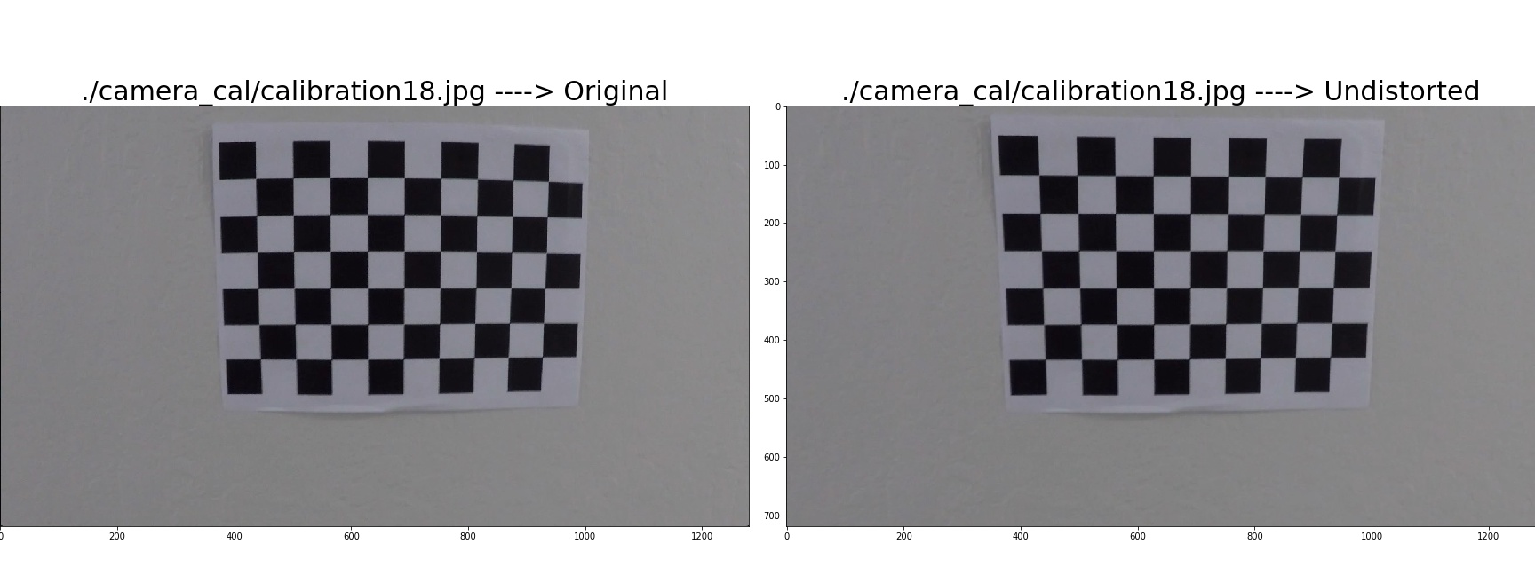 The camera calibration and distortion coefficients are stored using pickle to be used later.
The pipeline is contained in advanced_lane_detection.ipynb
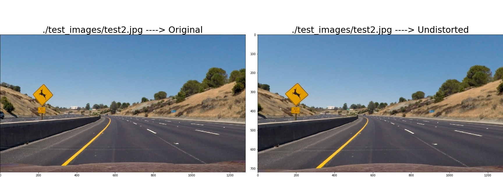
The camera calibration and distortion coefficients are loaded using pickle in Cell 2 of color_grad_threshold.ipynb. Following image shows the result of applying the calibration and undistortation to test2.jpg image shown in Cell 4 of color_grad_threshold.ipynb.
2. Describe how (and identify where in your code) you used color transforms, gradients or other methods to create a thresholded binary image. Provide an example of a binary image result.
The code to explore and evaluate color transforms and gradients is present in color_grad_threshold.ipynb.
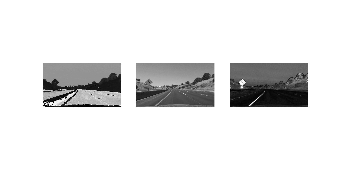
Following figure shows a test image in HLS with the three channels displayed seperately. It is clear that the S channel is important for further analysis as it shows the lane lines clearly. Code in Cell 6 of color_grad_threshold.ipynb.
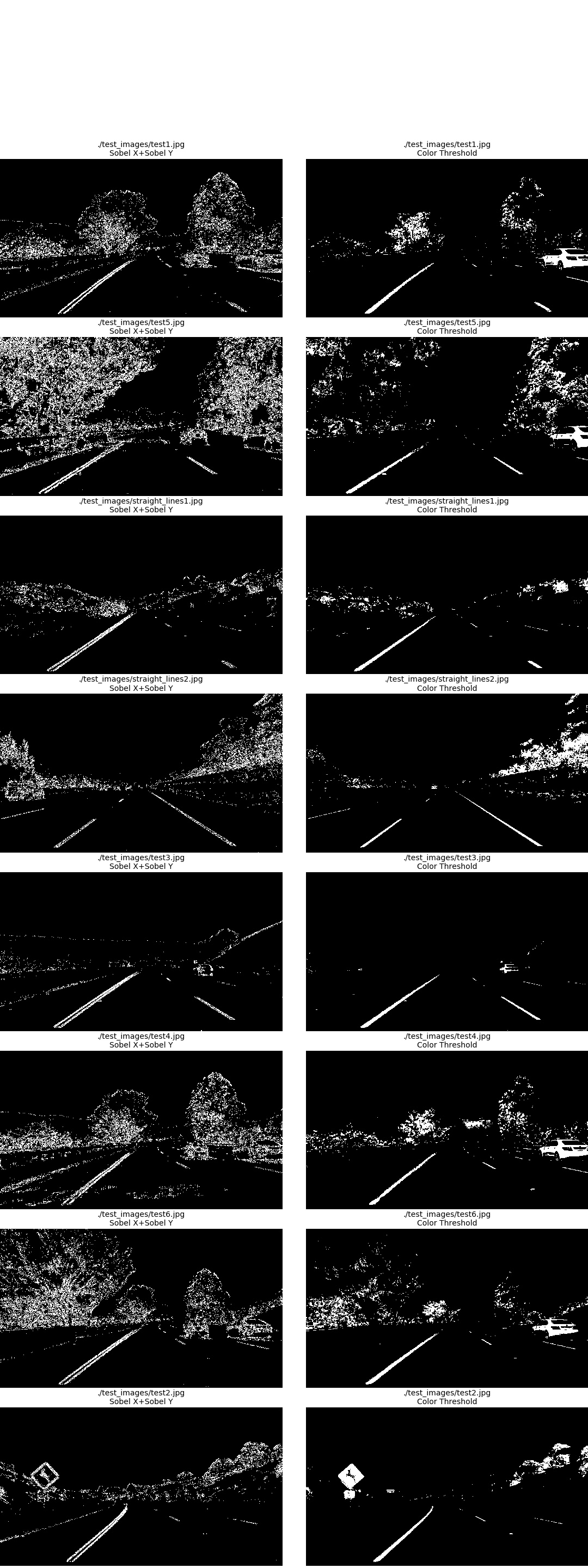
 Following this I computed Sobel X (Cell 8), Sobel Y (Cell 9), Magnitude (Cell 10), Color (Cell 11) and Direction threshold (Cell 12) images. I also calculated combined image of Sobel X + Sobel Y + Magnitude + Direcion (Cell 13). After some tweaking of the thresholds the following picture shows each of the thresholds for all the test images (Cell 14). You can see the lane lines in the combined image but it is still noisy and not very clear.
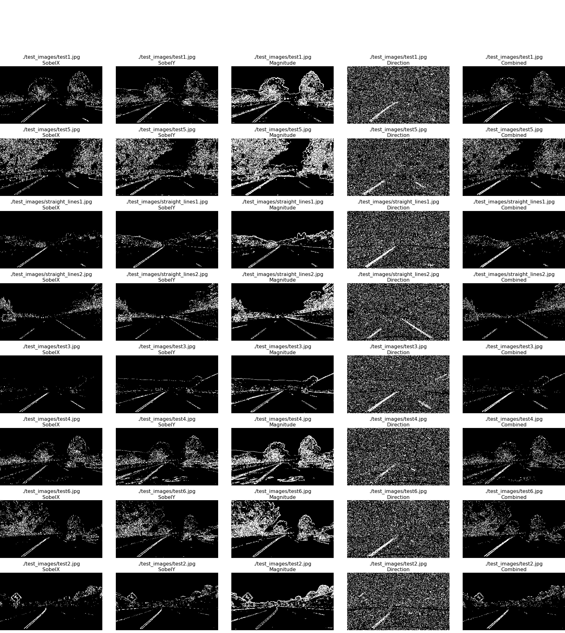 I observed that just Sobel X + Sobel Y performs well along with the Color threshold as see in Cell 10 of advanced_lane_detection.ipynb shown below. However the color threshold is still better. Hence, I have used just the color threshold in the rest of the project.
3. Describe how (and identify where in your code) you performed a perspective transform and provide an example of a transformed image.
My code for perspective transform is present in perspective_tranform.ipynb. I used test image with straignt lines - straignt_lines2.jpg for the transform. Four points are selected as shown on the image for the transform. The destination points were selected to get a clear picture of the street.
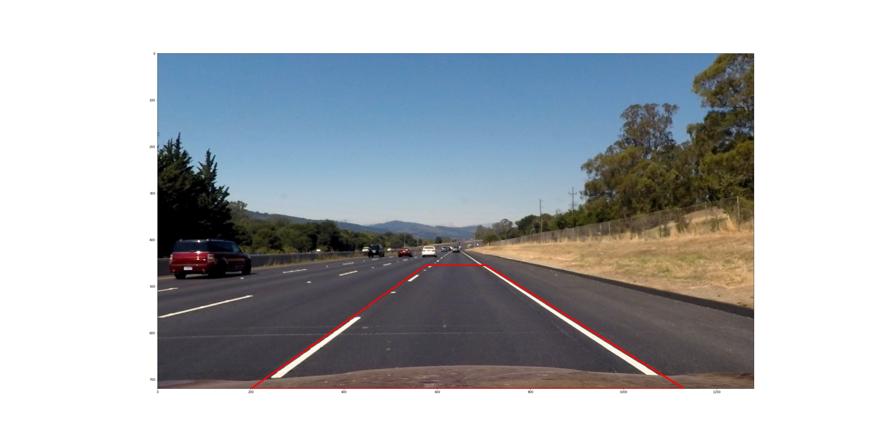 This resulted in the following source and destination points (Cell 5 of perspective_tranform.ipynb):
| Source | Destination |
|---|---|
| 200, 720 | 200, 720 |
| 1130, 720 | 1080, 720 |
| 705, 455 | 1080, 0 |
| 575, 455 | 200, 0 |
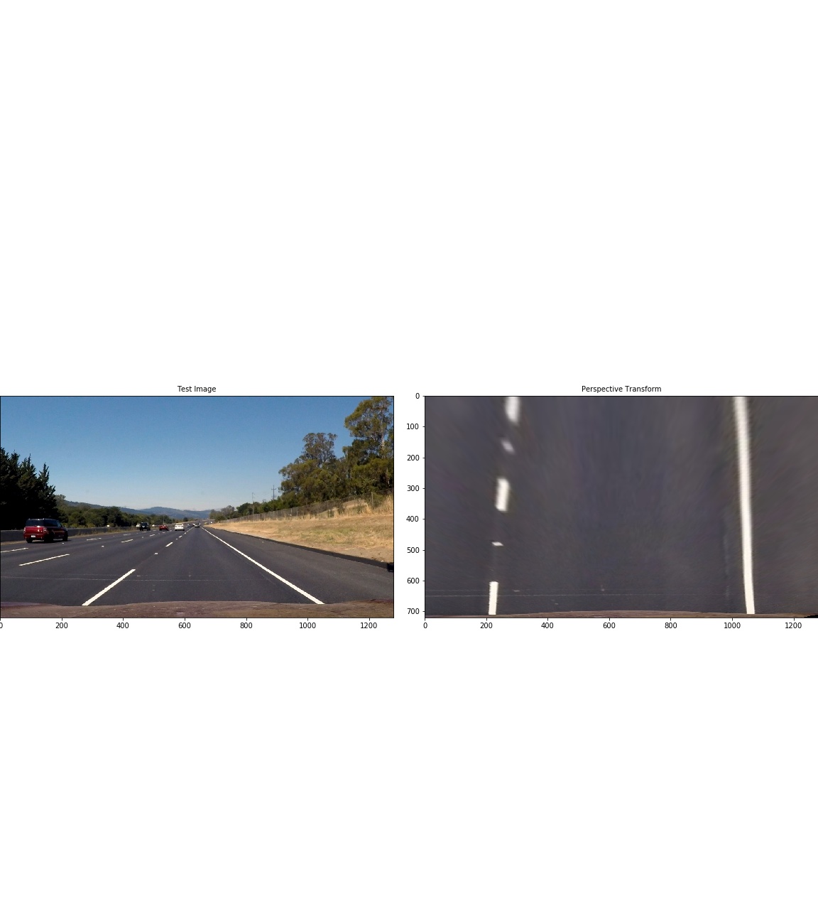
I used cv2.getPerspectiveTransform to create a transformation matrix and an inverse transformation matrix. Following figure shows the result of the transformation alongside the original (also Cell 5).
4. Describe how (and identify where in your code) you identified lane-line pixels and fit their positions with a polynomial?
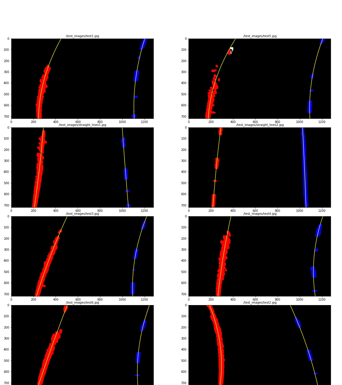
The code for lane line pixel detection is present in Cell 14 of advanced_lane_detection.ipynb. The code calculates the histogram of the bottom half of the image. Then it calculates the peaks of left and right half of the histogram. Each peak is the starting point of the left and right line. The code then identifies ten windows from which to identify lane pixels, each one centered on the midpoint of pixels from window below. Then a quadratic polynomial fit (np.polyfit()) is used to approximate the lane lines. In the same function another polynomial fit is performed on the same points converting pixels to meters which is used later for curvature calulation. Following picture demonstrates the binary images with identified points within the windows and polynomial fit lane lines.
5. Describe how (and identify where in your code) you calculated the radius of curvature of the lane and the position of the vehicle with respect to center.
This calculation is performed in Cell 16 of advanced_lane_detection.ipynb as following -
left_curverad = ((1 + (2 * left_fit_cr[0] * y_eval * ym_per_pix + left_fit_cr[1]) ** 2) ** 1.5) / np.absolute(2 * left_fit_cr[0])
right_curverad = ((1 + (2 * right_fit_cr[0] * y_eval * ym_per_pix + right_fit_cr[1]) ** 2) ** 1.5) / np.absolute(2 * right_fit_cr[0])
Here left_fit_cr and right_fit_cr is the array containing the polynomial, y_eval is the maxY value and ym_per_pix is the meter per pixel value.
The vehicle position is calculated in Cell 19 of advanced_lane_detection.ipynb as follows -
- Calculate vehicle center by tranforming the image center from pixels to meters
- Calculate the lane center by evaluating the left and right lane polynomial at max Y and finding their midpoint
- The sign between the lane center and vehicle center tells us if the vehicle is left or right of center
6. Provide an example image of your result plotted back down onto the road such that the lane area is identified clearly.
This code is implemented in function pic_pipeline() located in Cell 19 of advanced_lane_detection.ipynb. Cell 20 calls this function for all test images and provides following result.
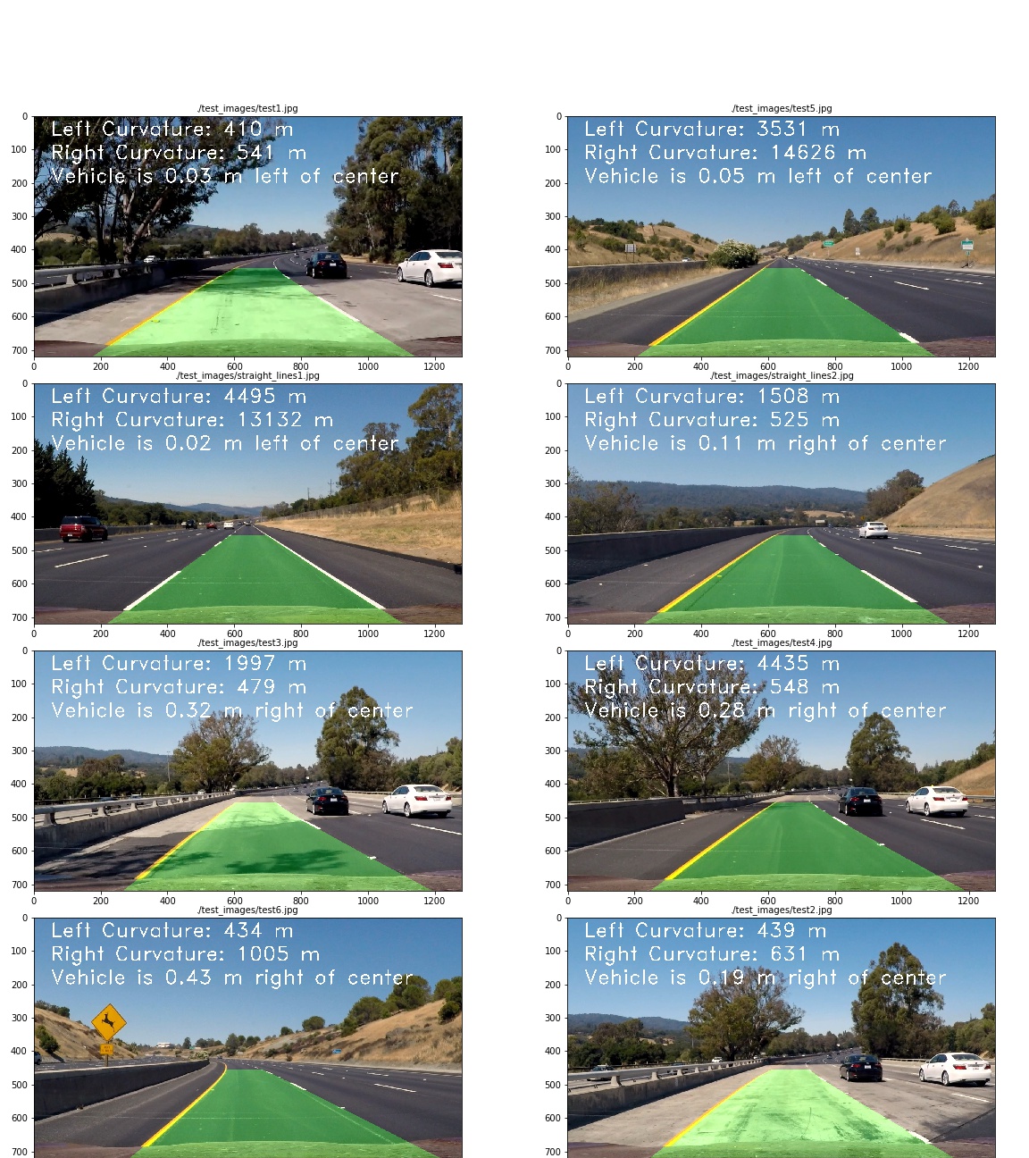
1. Provide a link to your final video output. Your pipeline should perform reasonably well on the entire project video (wobbly lines are ok but no catastrophic failures that would cause the car to drive off the road!).
The video_pipeline() simply calls the pic_pipeline() for every frame in the video as shown in Cell 22 of advanced_lane_detection.ipynb. The result video is present here. The pipeline does a fairly good job for the entire video.
1. Briefly discuss any problems / issues you faced in your implementation of this project. Where will your pipeline likely fail? What could you do to make it more robust?
I had to spend by far the longest time coming up with the right color transform. This made me really appreaciate the CNN and deep learning techniques we used in the previous project.
When I started off I was using a combined binary of the following SobelX + SobelY + Direction + Magnitude. Then I switched to a SobelX+SobelY combined image and I was using thresh_min=20, thresh_max=160 for SobelX and SobelY. This was not detecting the right hand lane line is fram 616 to of the image. After playing around with it further I lowered the thresh_min to 8 which produced acceptable result for the frame. However, still the frames 1039 and 1040 were incorrectly detecting the right lane in the middle of the lane. This was because the binary image for those misdetected tree shadows as lane lines. Based on suggestion from previous reviewer I implemented a color threshold to specifically identify yellow and white colors for the lanes using color masks as shown in Cell 11 of color_grad_threshold.ipynb. To the best of my knowledge this has fixed the issues and the project video result.
I did not spend time to improve results for challenge videos in the interest of time and my pipeline did not perform well on them.
Following improvements can be made to improve the pipeline for challenge videos -
- Information from the previous frame may be used for robust and perhaps faster predictions.
- Outlier rejection and a low-pass filters may be added for smooth predictions.
- Other image thresholds could perhaps be used to improve detection.
- If the lane detection is wrong for a particular frame it can be rejected and the previous prediction may be used.
- Spline or higher order polynomial may be used fit a lane line through the binary image.
