Advanced Lane Finding Project
The goals / steps of this project are the following:
- Compute the camera calibration matrix and distortion coefficients given a set of chessboard images.
- Apply a distortion correction to raw images.
- Use color transforms, gradients, etc., to create a thresholded binary image.
- Apply a perspective transform to rectify binary image ("birds-eye view").
- Detect lane pixels and fit to find the lane boundary.
- (To optimize: Only for videos after analyzing the first image) Detect lane pixels around the detected line of the previous image.
- Determine the curvature of the lane and vehicle position with respect to the center.
- Warp the detected lane boundaries back onto the original image.
- Output visual display of the lane boundaries and numerical estimation of lane curvature and vehicle position.
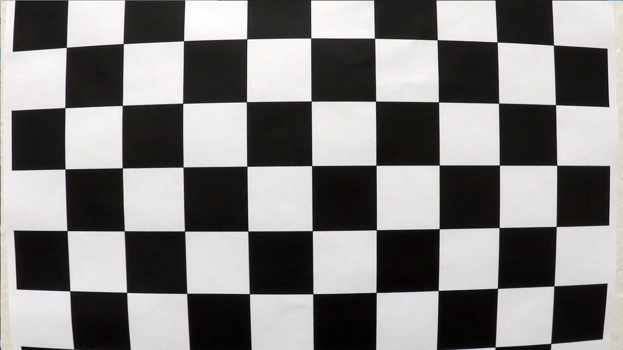
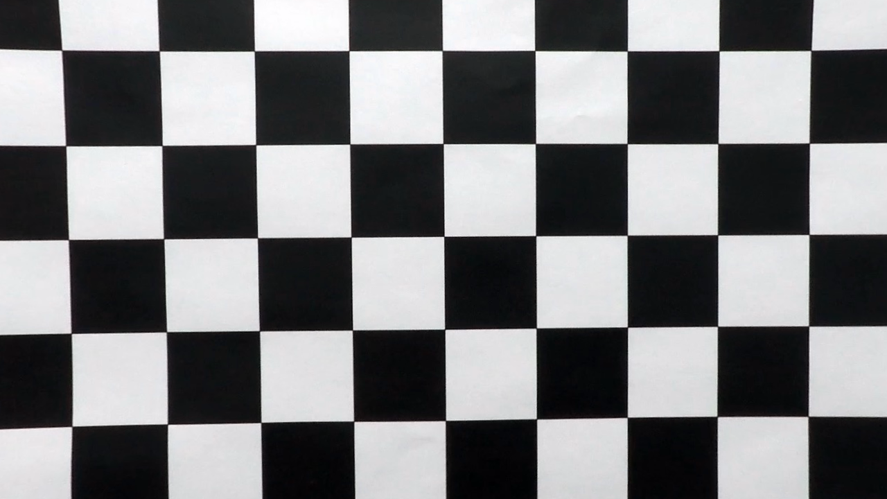
1. Computation of the camera matrix and distortion coefficients with an example of distortion corrected calibration image.
The code for this step is called Camera_calibration.py.
I start by preparing "object points", which will be the (x, y, z) coordinates of the chessboard corners in the world.
Here I am assuming the chessboard is fixed on the (x, y) plane at z=0, such that the object points are the same for each calibration image.
Thus, objp is just a replicated array of coordinates, and objpoints will be appended with a copy of it every time I successfully detect all chessboard corners in a test image.
imgpoints will be appended with the (x, y) pixel position of each of the corners in the image plane with each successful chessboard detection.
I then used the output objpoints and imgpoints to compute the camera calibration and distortion coefficients using the cv2.calibrateCamera() function.
I also save these two matrixes using np.savez such that I can use them later.
Then, I applied this distortion correction to the test image using the cv2.undistort() function and obtained this result:
| Original image | undistorted image |
|---|---|
 |
 |
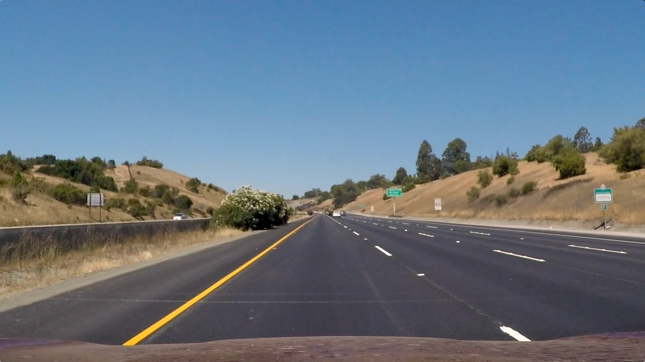
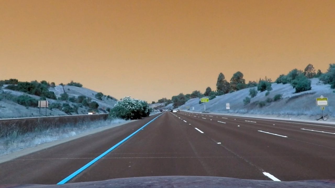
The code for this step is called Line_detection_advanced.py.
Initially, it loads mtx, and dist matrices from the camera calibration step.
Using the saved mtx, dist from calibration, I have undistorted an image from a road:
| Original image | undistorted image |
|---|---|
 |
 |
(TODO: Which line of code?)
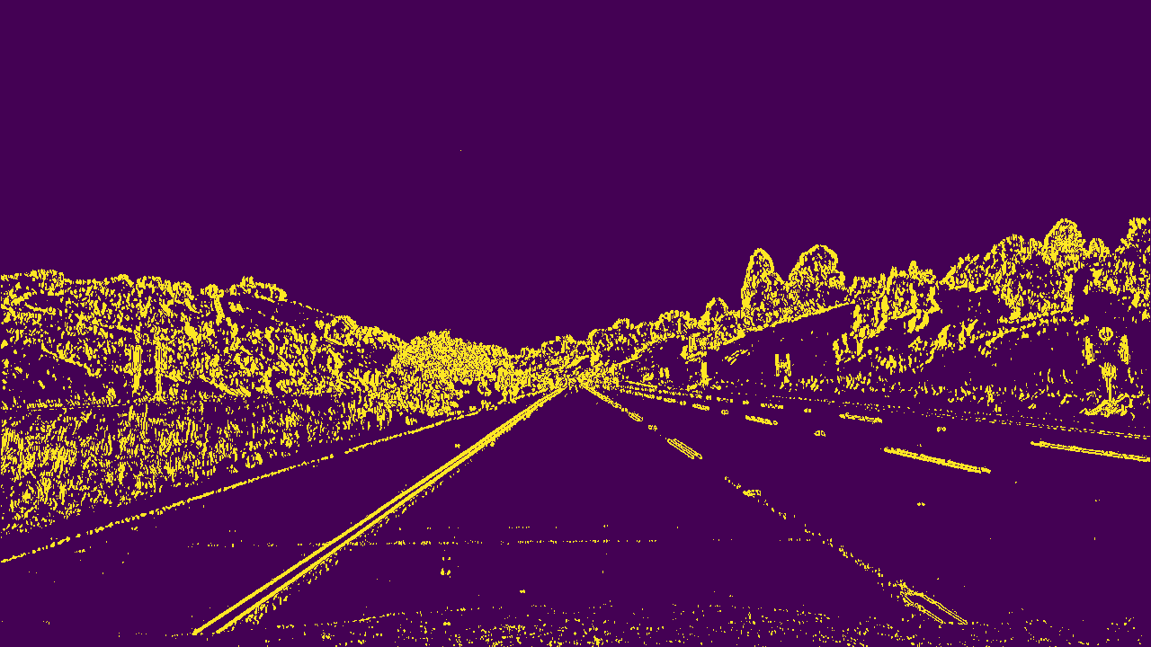
I used a combination of color and gradient thresholds to generate a binary image (thresholding steps at lines 30 through 53 in Line_detection_advanced.py).
For gradient thresholds, the code includes a function called grad_thresh.
First, I converted the image into grayscale cv2.cvtColor(img, cv2.COLOR_BGR2GRAY). Note that if you are using cv2.imread, you should use cv2.COLOR_BGR2GRAY.
But if you are using matplotlib.image.imread, you should use cv2.COLOR_BGR2GRAY.
Then, I took the derivative in the x-direction, using cv2.Sobel (Why? Because vertical lines can be detected better using gradient in the horizontal direction).
Then, I scaled its magnitude into 8bit 255*np.absolute(sobelx)/np.max(abs_sobelx), and conervetd to np.unit8.
In the end, to generate the binary mage, I used np.zeros_like, and applied the threshold.
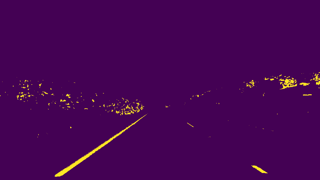
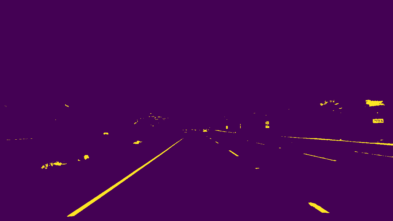
For color threshhold, the code includes a function called color_thresh. I used HLS colorspace using cv2.cvtColor(img, cv2.COLOR_BGR2HLS).
(Why? because yellow and white colors can be detected well in S space).
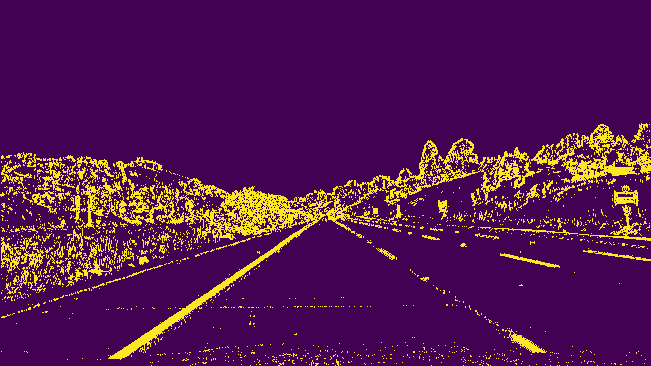
Then, I created the binary image np.zeros_like, and applied the threshold on the S channel. Also, I have applied the threshold on R space in RGB colorspace. The results are as follows:
| Gradient threshhold | S threshhold (HSV) | R threshhold from (RGB) |
|---|---|---|
 |
 |
 |
In the end, I have combined the two binary thresholds, and here is an example of my output for this step.
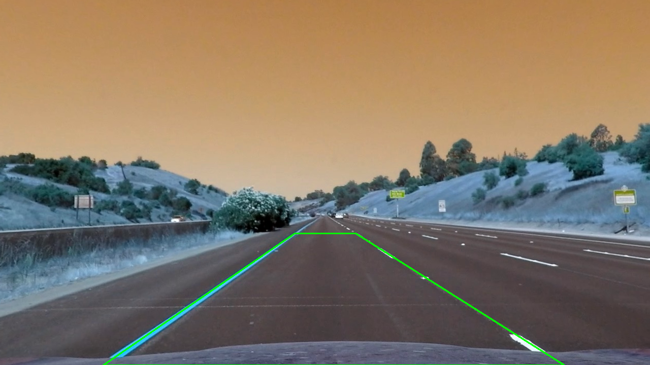
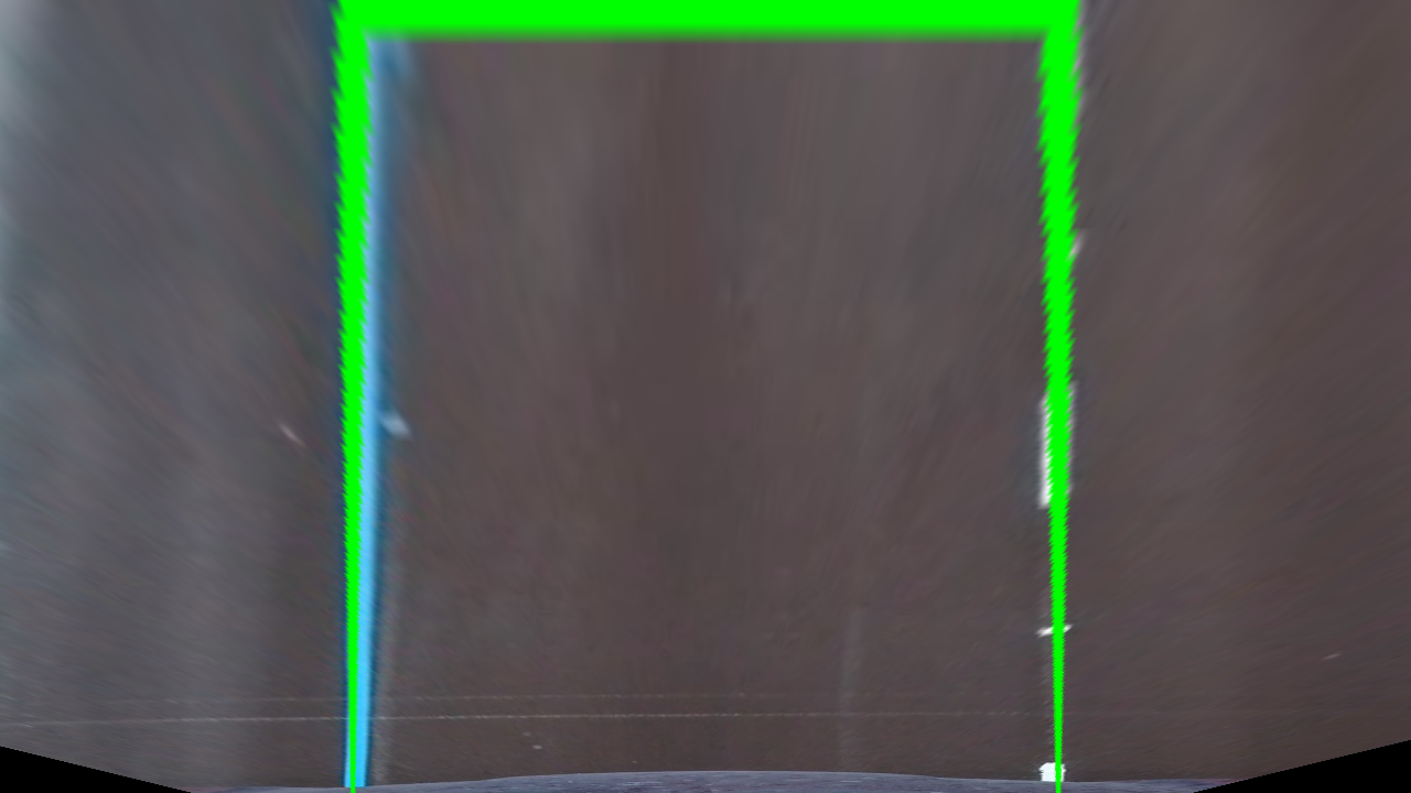
The code for my perspective transform includes a function called warp(), which appears in lines 55 through 68 in the file Line_detection_advanced.py.
The warp() function takes as inputs an image (img), as well as source (src) and destination (dst) points.
I chose the hardcode the source and destination points in the following manner:
src = np.float32(
    [[(img_size[0] / 2) - 55, img_size[1] / 2 + 100],
    [((img_size[0] / 6) - 10), img_size[1]],
    [(img_size[0] * 5 / 6) + 60, img_size[1]],
    [(img_size[0] / 2 + 55), img_size[1] / 2 + 100]])
dst = np.float32(
    [[(img_size[0] / 4), 0],
    [(img_size[0] / 4), img_size[1]],
    [(img_size[0] * 3 / 4), img_size[1]],
    [(img_size[0] * 3 / 4), 0]])
This resulted in the following source and destination points:
| Source | Destination |
|---|---|
| 585, 460 | 320, 0 |
| 203, 720 | 320, 720 |
| 1127, 720 | 960, 720 |
| 695, 460 | 960, 0 |
I verified that my perspective transform was working as expected by drawing the src and dst points onto a test image and its warped counterpart to verify that the lines appear parallel in the warped image.
| Original image | undistorted image |
|---|---|
 |
 |
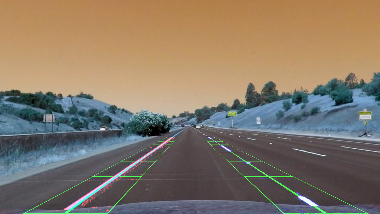
To find lane pixels, a function called find_lane_pixels() is defined.
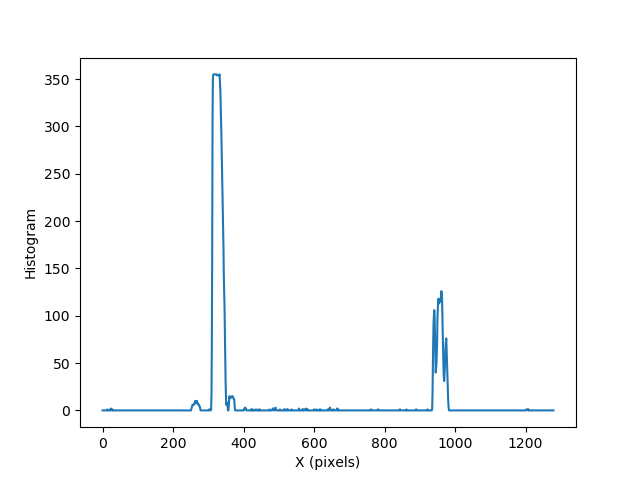
First, the histogram of the bottom half of the image along the vertical axis is computed using npsum.
Then the peaks in the left half side and right half side of the histogram are computed as the initial estimate of the left and right lines respectively.
Then, the number of sliding windows nwindows and horizontal margin margin and the minimum number of pixels minpix are specified.
Then to recognize the left and right lines pixel positions, I defined a for loop.
To optimize the search process, at every iteration, the horizontal position of the center of the left and right windows is passed to the next iteration to find the boundaries of the next window.
I start processing the bottom windows.
The vertices of each left and right window are computed. The indices of nonzero pixels in x and y directions within the windows are identified.
To visualize this step, the left and right rectangles are plotted on the image using cv2.rectangle by specifying two opposite vertices of a rectangle.
I append indices to the main lists of indices, using np.append.
If the minimum number of recognized indices in the left and right lists are more than minpix, I update the position of the center of the left and right windows.
I continue to process the next window which is the window above the bottom window. I continue processing each window to reach the nwindows.
After the loop ends, I concatenate the arrays of indices (previously was a list of lists of pixels), using np.concatenate.
Finally, I extract the left and right line pixel positions as the output of find_lane_pixels() function.
The next step is to fit a 2nd order polynomial using fit = np.polyfit to the output of the previous function find_lane_pixels.
To do this, I defined a function called fit_polynomial().
To draw polynomials on the image, first I generate x and y values for plotting, using np.linspace.
Then I used fit[0]*ploty**2 + fit[1]*ploty + fit[2] to have all points on the line for left and right lines, seperately.
To plot them on the image, I use plt.plot. Also, I visualize the whole left and right windows on the images.
The output of the last function is the following figure:
| Binary image | Road image |
|---|---|
 |
4.2 Detect lane pixels around the detected line. (To optimize: Only for videos after analyzing the first image)
For analyzing videos, we can use the detected lane lines information from the previous image to speed the code.
To do this, I have defined a function called search_around_poly.
The input is the polynomial coefficient of the previous image, and a margin to restrict the area around the line for a search.
(Why? Because the lane lines do not usually jump! )
The output for this section is as follows:
5. Calculate the radius of curvature of the lane and the position of the vehicle with respect to the center.
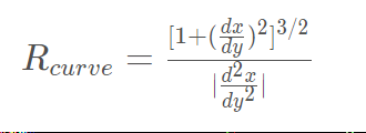
I have defined a function called measure_curvature_real to measure the radius of curvature in meters.
The input to the function is the output of the fit_polynomial() function, explinaed in the previus section. The formula is given below:
To calculate the position of the car with respect to the center of the lane, I have assumed that the camera is placed in the middle of the car.
Then the position of the middle of the lane is calculated as the mean value of the detected left and right lines on the bottom of the image.
The center of the car or camera is calculated by the image size, using image.shape[1].
Then the off-center pixel is the distance between these two numbers, which is then converted to meters.
These two numbers are plotted on the images using cv2.putText.
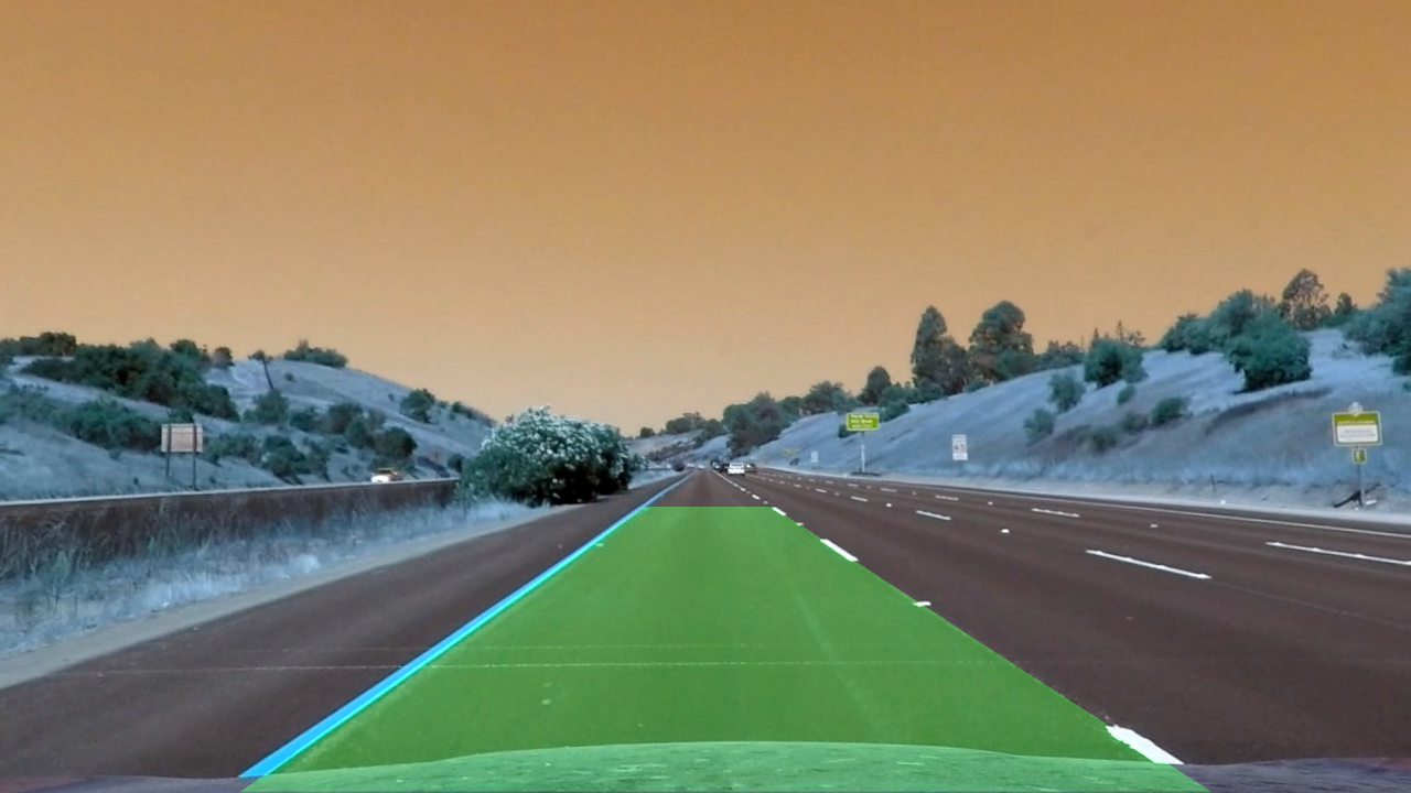
6. Provide an example image of your result plotted back down onto the road such that the lane area is identified clearly.
I implemented this step in lines # through # in my code in yet_another_file.py in the function map_lane().
Here is an example of my result on a test image:
1. Provide a link to your final video output. Your pipeline should perform reasonably well on the entire project video (wobbly lines are ok but no catastrophic failures that would cause the car to drive off the road!).
Here's a link to my video result
1. Briefly discuss any problems/issues you faced in your implementation of this project. Where will your pipeline likely fail? What could you do to make it more robust?
Here I'll talk about the approach I took, what techniques I used, what worked and why, where the pipeline might fail and how I might improve it if I were going to pursue this project further.
This is a project from the Udacity Self Driving car course (https://github.com/udacity/CarND-Advanced-Lane-Lines).
