The goals / steps of this project are the following:
- Compute the camera calibration matrix and distortion coefficients given a set of chessboard images.
- Apply a distortion correction to raw images.
- Use color transforms, gradients, etc., to create a thresholded binary image.
- Apply a perspective transform to rectify binary image ("birds-eye view").
- Detect lane pixels and fit to find the lane boundary.
- Determine the curvature of the lane and vehicle position with respect to center.
- Warp the detected lane boundaries back onto the original image.
- Output visual display of the lane boundaries and numerical estimation of lane curvature and vehicle position.
The code for this step is contained in camera_cal.py
I start by preparing "object points", which will be the (x, y, z) coordinates of the chessboard corners in the world. Here I am assuming the chessboard is fixed on the (x, y) plane at z=0, such that the object points are the same for each calibration image. Thus, objp is just a replicated array of coordinates, and objpoints will be appended with a copy of it every time I successfully detect all chessboard corners in a test image. imgpoints will be appended with the (x, y) pixel position of each of the corners in the image plane with each successful chessboard detection.
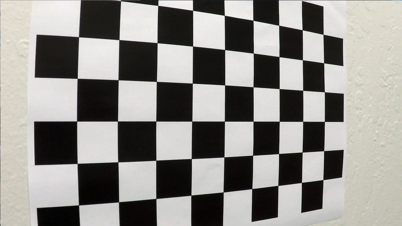
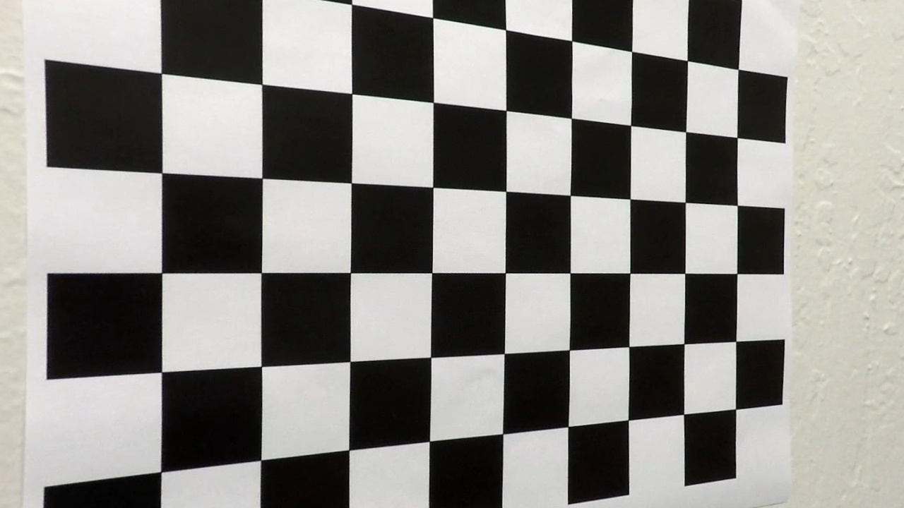
I then used the output objpoints and imgpoints to compute the camera calibration and distortion coefficients using the cv2.calibrateCamera() function. I applied this distortion correction to the test image using the cv2.undistort() function and obtained this result:
The camera matrix and distortion coefficient are saved in dis_pickle.p for loading in future image and video processing.
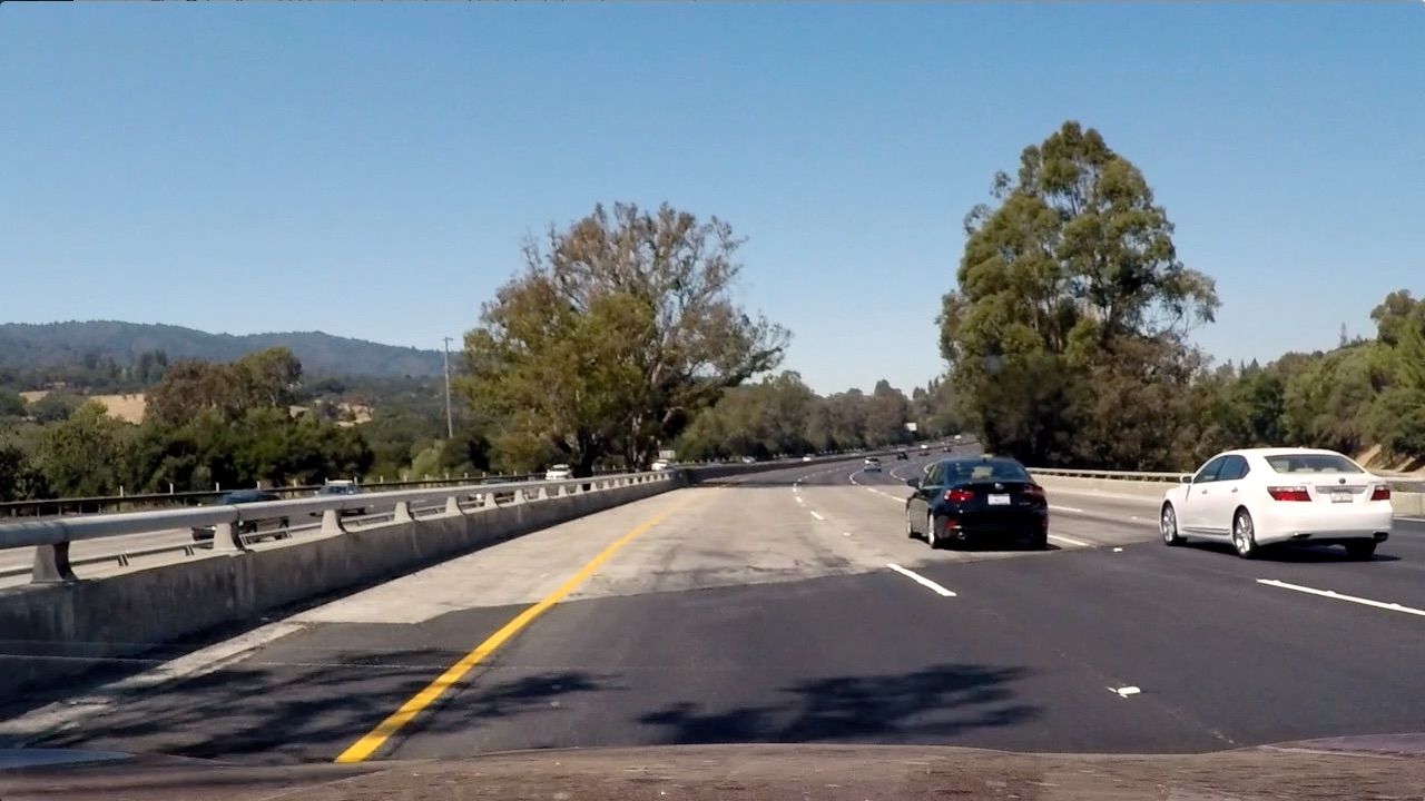
To demonstrate this step, I will describe how I apply the distortion correction to one of the test images like this one:
The distortion coefficient and camera matrix are loaded from dis_pickle.p in main.py with
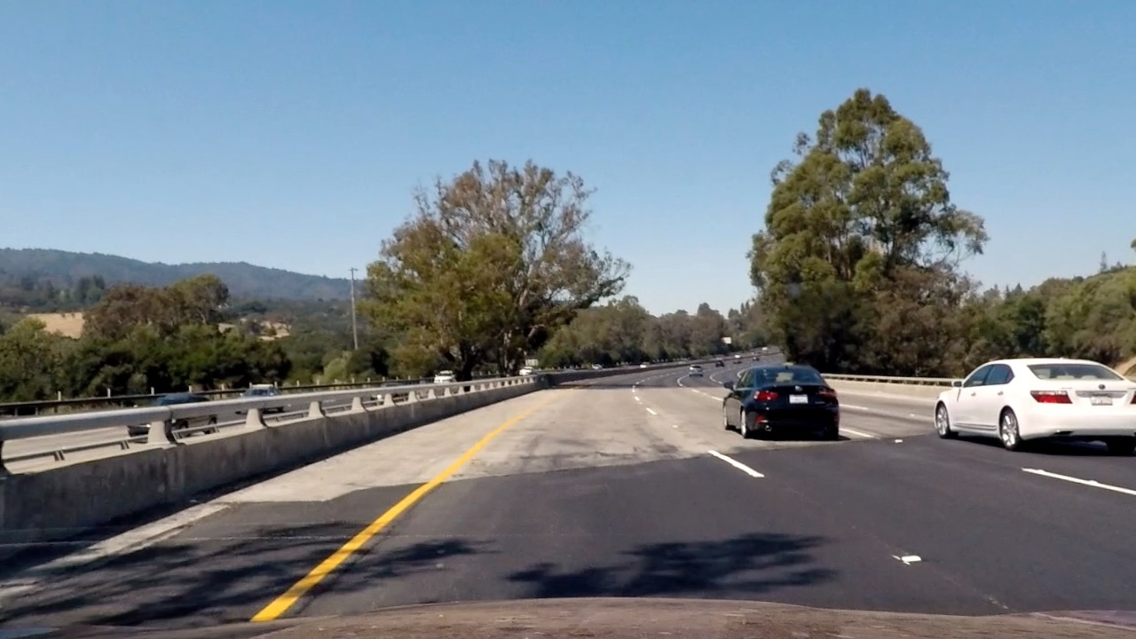
mtx, dist = read_discortion_coefficient()The above parameters are then applied to the image test image test4.jpg in test_images and undistorted produced the below output:
The slight difference can be observed from the edges of the images.
In pipeline function in main.py, I used cv2.Sobel on the L channel and take the abcolute value of sobel output. The abcolute value is then thresholded between 170 and 255.
The second processing method I used is color thresholding. This method can be utilized to identify yellow lane lines under sunshines. The threshold parameters are chosen to be 20 and 100.
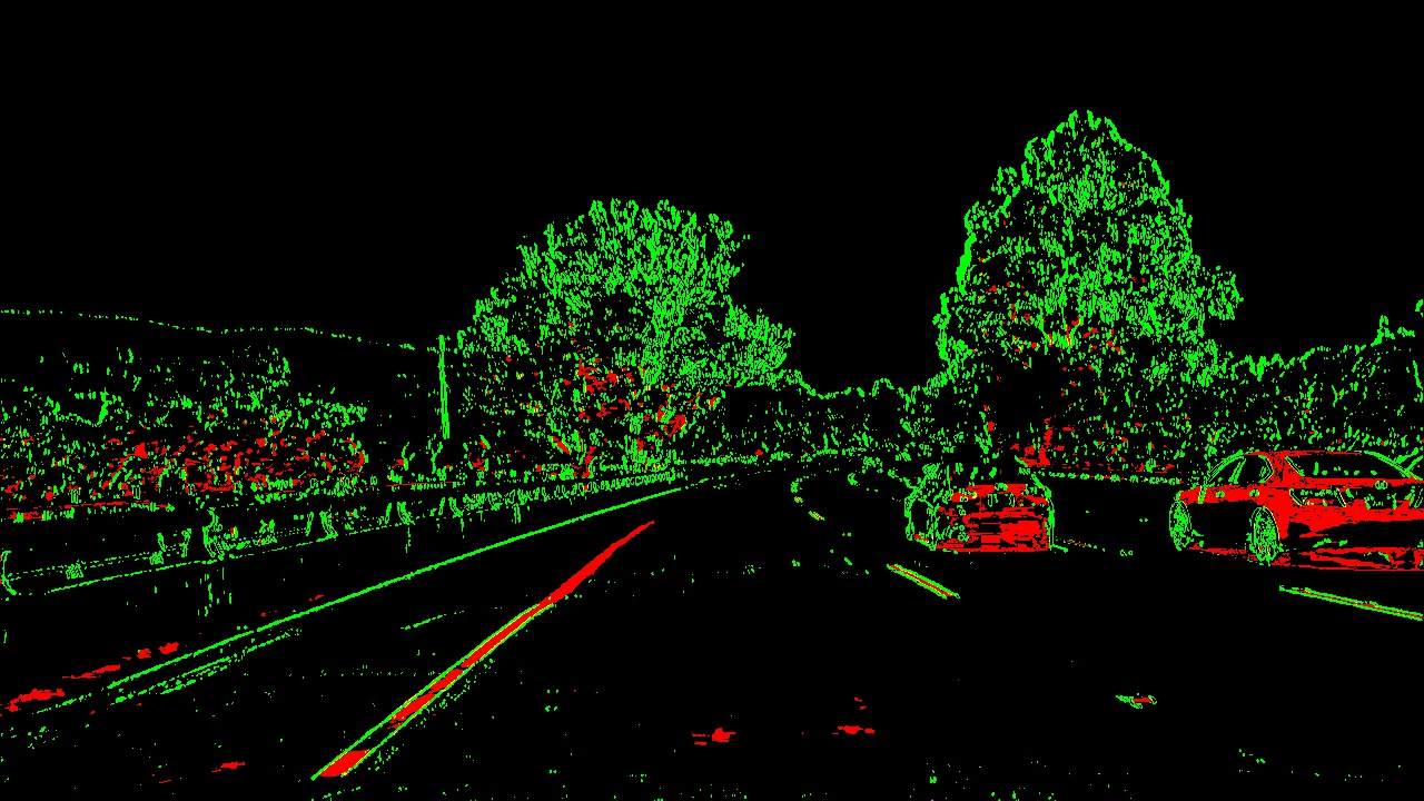
The identified edges are outlines in different colors in the below imnage. Different colors tells me which filter is better at identifying which part of the lanes and helps adjusting the threshold values.
Below is the demonstration of the thresholded image:
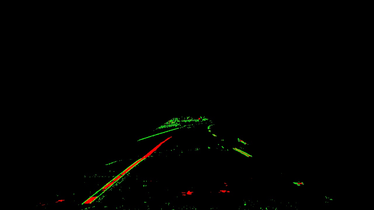
A lot of unnecessary lines are presented in the above image and not contributing to lane detection. This is solved by applying a mask on the above image with the following regions of interest:
mask_region = np.array([[(100, 720), (600, 400), (700, 400), (1200, 720)]], dtype=np.int32)The perpective transform funcion is included in corners_unwarp
src = np.float32([[(200, 720), (570, 470), (720, 470), (1130, 720)]])
dst = np.float32([[(350, 720), (350, 0), (980, 0), (980, 720)]])
This resulted in the following source and destination points:
| Source | Destination |
|---|---|
| 200, 720 | 350, 720 |
| 570, 470 | 350, 0 |
| 720, 470 | 980, 0 |
| 1130, 720 | 980, 720 |
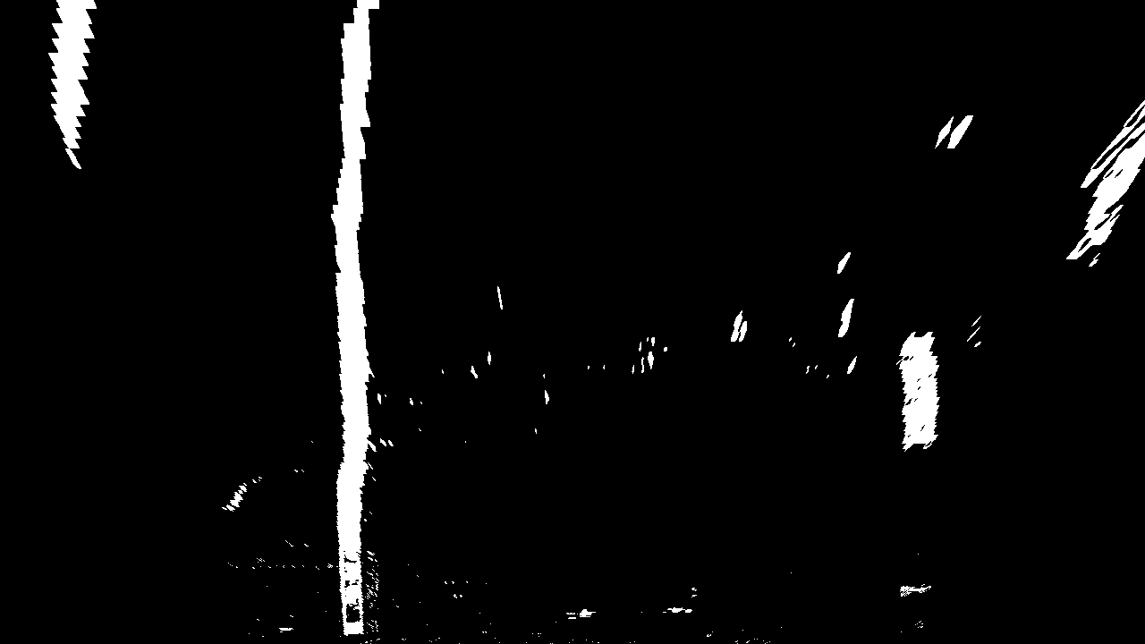
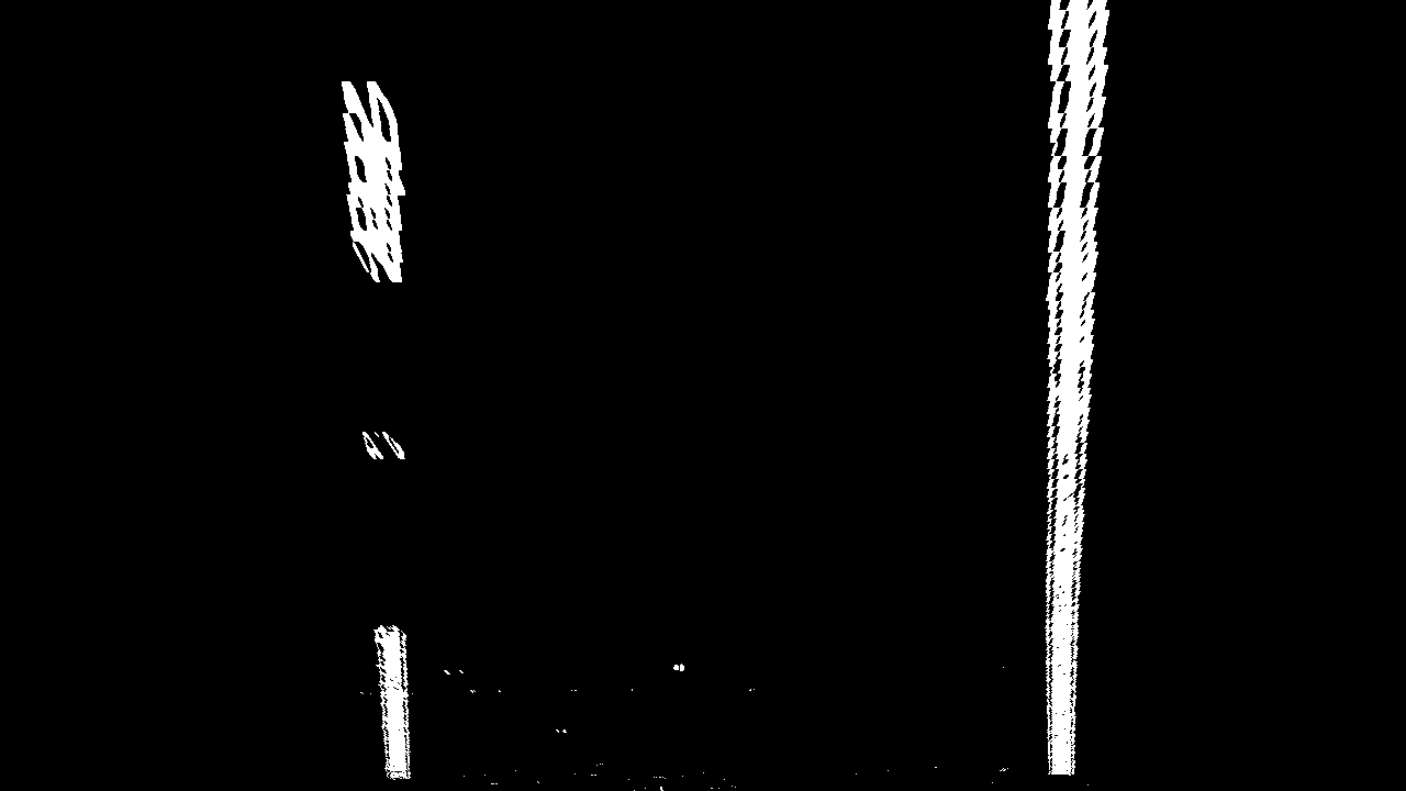
I verified that my perspective transform was working as expected by drawing the src and dst points onto a test image and its warped counterpart to verify that the lines appear parallel in the warped image.
Although it is not farily obvious because the right lane is small and short, but the parallelism can still be observed. Test on another image with equal length of left and right lanes produces better result:
In process_image function, I first undistort and perspective trandorm the input frame, then generate histogram on the pixel data with the following code block
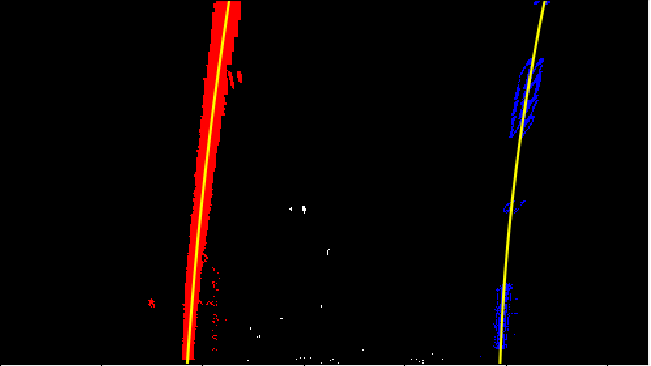
histogram = np.sum(binary_warped[int(binary_warped.shape[0]/2)::axis=0)The peak value in the histogram is saved as middle point of left and right lane where most white pixels exist. Then, a sliding window search is applied starting at the middle point detected in the histogram. If ther number of pixels in the windows exceeds "50", the pixels in this window is classified as lane pixels.
One notable trick is in order to accelerate the later frames, the previous positions are saved and used as search starting point in the later frames. This is because lane position usually doesn't vary by much in consecutive frames.
The polynomial fitting is done by polyfit function:
left_fit_cr = np.polyfit(lefty * ym_per_pix, leftx * xm_per_pix, 2)
right_fit_cr = np.polyfit(righty * ym_per_pix, rightx * xm_per_pix, 2)
where
ym_per_pix
xm_per_pix
are the scaling factor for pixel to meters convertoin in x and y axis.
The curvature calculation is done with the help of
ym_per_pix
xm_per_pix
The calculations are doen in process_image in the following code block:
ploty = np.linspace(0, binary_warped.shape[0] - 1, binary_warped.shape[0])
y_eval = np.max(ploty)
left_fit_cr = np.polyfit(lefty * ym_per_pix, leftx * xm_per_pix, 2)
right_fit_cr = np.polyfit(righty * ym_per_pix, rightx * xm_per_pix, 2)
left_curverad = ((1 + (2 * left_fit_cr[0] * y_eval * ym_per_pix + left_fit_cr[1]) ** 2 ** 1.5) / np.absolute(2 * left_fit_cr[0])
right_curverad = ((1 + (2 * right_fit_cr[0] * y_eval * ym_per_pix + right_fit_cr[1]) ** 2) ** 1.5) / np.absolute(2 * right_fit_cr[0])
average_curvature = (left_curverad + right_curverad)/2
In order to calculate the car offset from the middle of the lane, an assumption is used: the camera is at the middle of the car. Because each frame is 720x1280, the middle of the car is at pixel 640. Computing the middle pixel position of left and right lane and take the absolute value between 640 produces the pixel offset of car compared to the middle of the lane. This value is then scaled by xm_per_pix because the offset is on x axis.
left_lane_buttom_x = left_fit[0]*719**2 + left_fit[1]*719 + left_fi[2]
right_lane_buttom_x = right_fit[0]*719**2 + right_fit[1]*719 + right_fit[2]
mid_lane_x = (left_lane_buttom_x + right_lane_buttom_x)/2
vehicle_offset_x = abs(mid_lane_x - 640) # in pixels
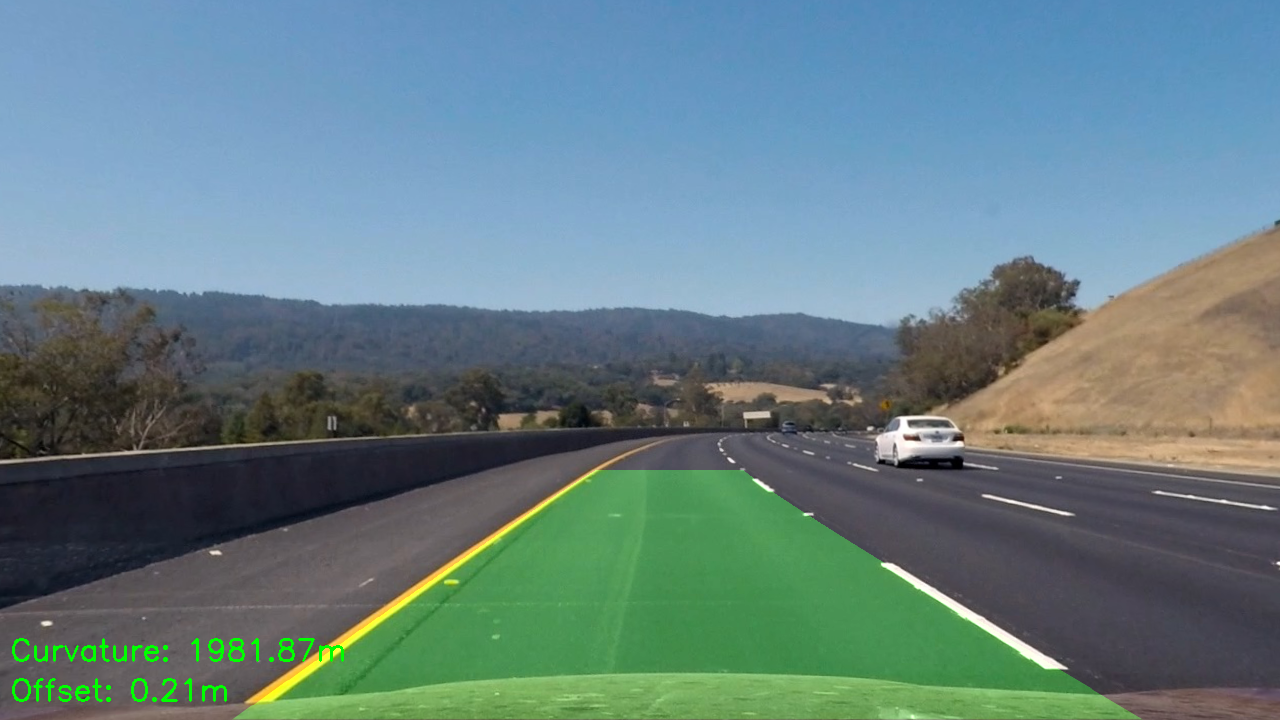
vehicle_offset_x_meters = vehicle_offset_x * xm_per_pixThe mapping overlay is done by ploting on the perspective transformed image and then reverse transform back to the actual view perspective:
# Create an image to draw the lines on
warp_zero = np.zeros_like(binary_warped).astype(np.uint8)
color_warp = np.dstack((warp_zero, warp_zero, warp_zero))

# Recast the x and y points into usable format for cv2.fillPoly()
pts_left = np.array([np.transpose(np.vstack([left_fitx, ploty]))])
pts_right = np.array([np.flipud(np.transpose(np.vstack([right_fitx, ploty])))])
pts = np.hstack((pts_left, pts_right))

# Draw the lane onto the warped blank image
cv2.fillPoly(color_warp, np.int_([pts]), (0,255, 0))

# Warp the blank back to original image space using inverse perspective matrix (Minv)
newwarp = cv2.warpPerspective(color_warp, np.linalg.inv(perspective_matrix), (image.shape[1], image.shape[0]))
# Combine the result with the original image
result = cv2.addWeighted(undist, 1, newwarp, 0.3, 0)

# Curverture
cv2.putText(result, "Curvature: " + str(float("{0:.2f}".format(average_curvature))) + "m", curvature_position, font, fontScale, fontColor, lineType)
v2.putText(result, "Offset: " + str(float("{0:.2f}".format(vehicle_offset_x_meters))) + "m", offset_position, font, fontScale, fontColor, lineType)Here's a link to video
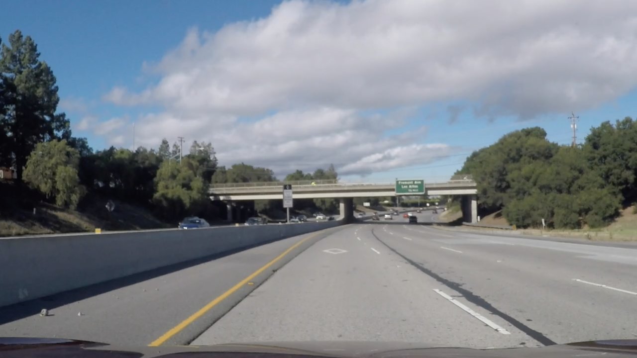
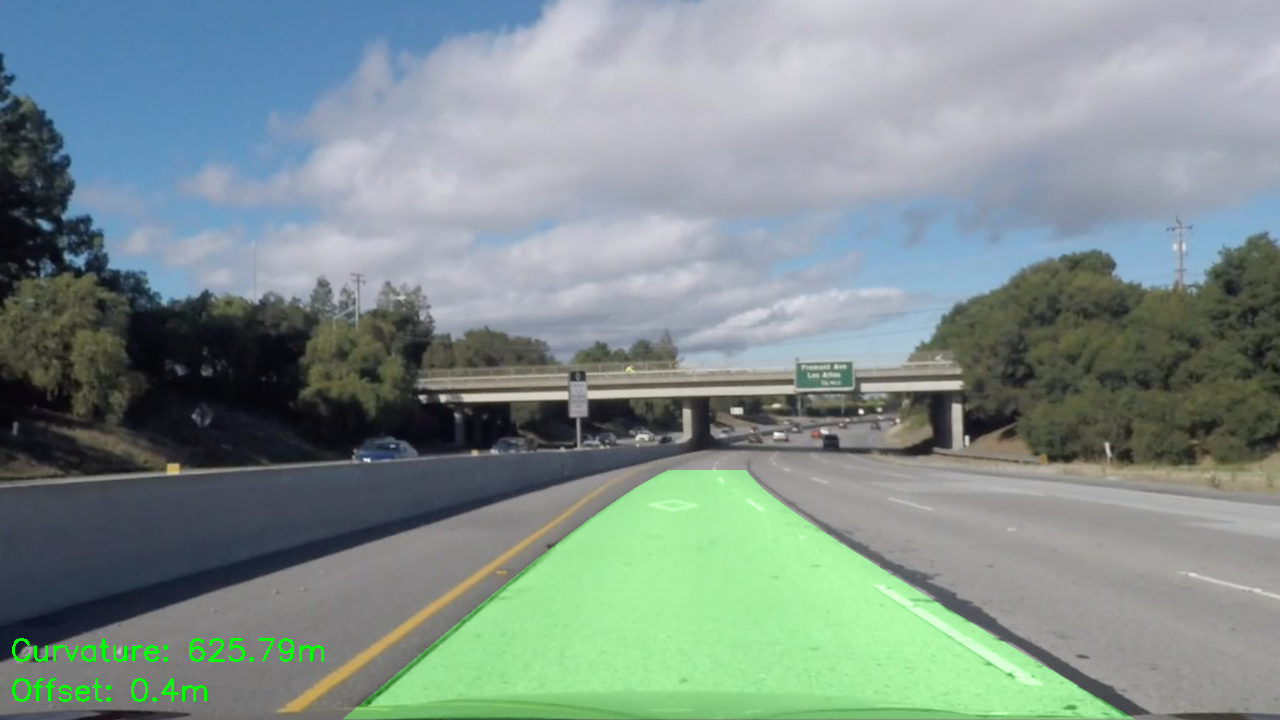
This algorithm works perfectely on the original video. However, under different conditions it might fail pretty badly. For example, if the rode is not clean the algorithm might misclassify the non-lane component as lane:
The left lane is not detected correctly because of the gap between road materials creates a black straight line
The above issue can be resolved by adjusting thresholding values and the use of multiple thresholding techniques in combination. For example, the yellow lane can be differentiated by using different color thresholding values.
