Berkanktk / Algorithm-visualizer

Visualize key computer science algorithms, including sorting, searching, mazegen, pathfinding, and data structures, in an interactive and user-friendly way.

Algorithm Visualizer

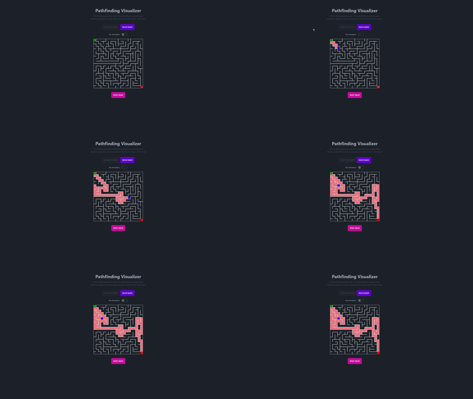
This repository contains a dynamic and interactive visualizer for a wide array of algorithms and data structures. It's designed to provide a clear and educational insight into how different algorithms and data structures work under the hood.

Try it out!

List of Contents

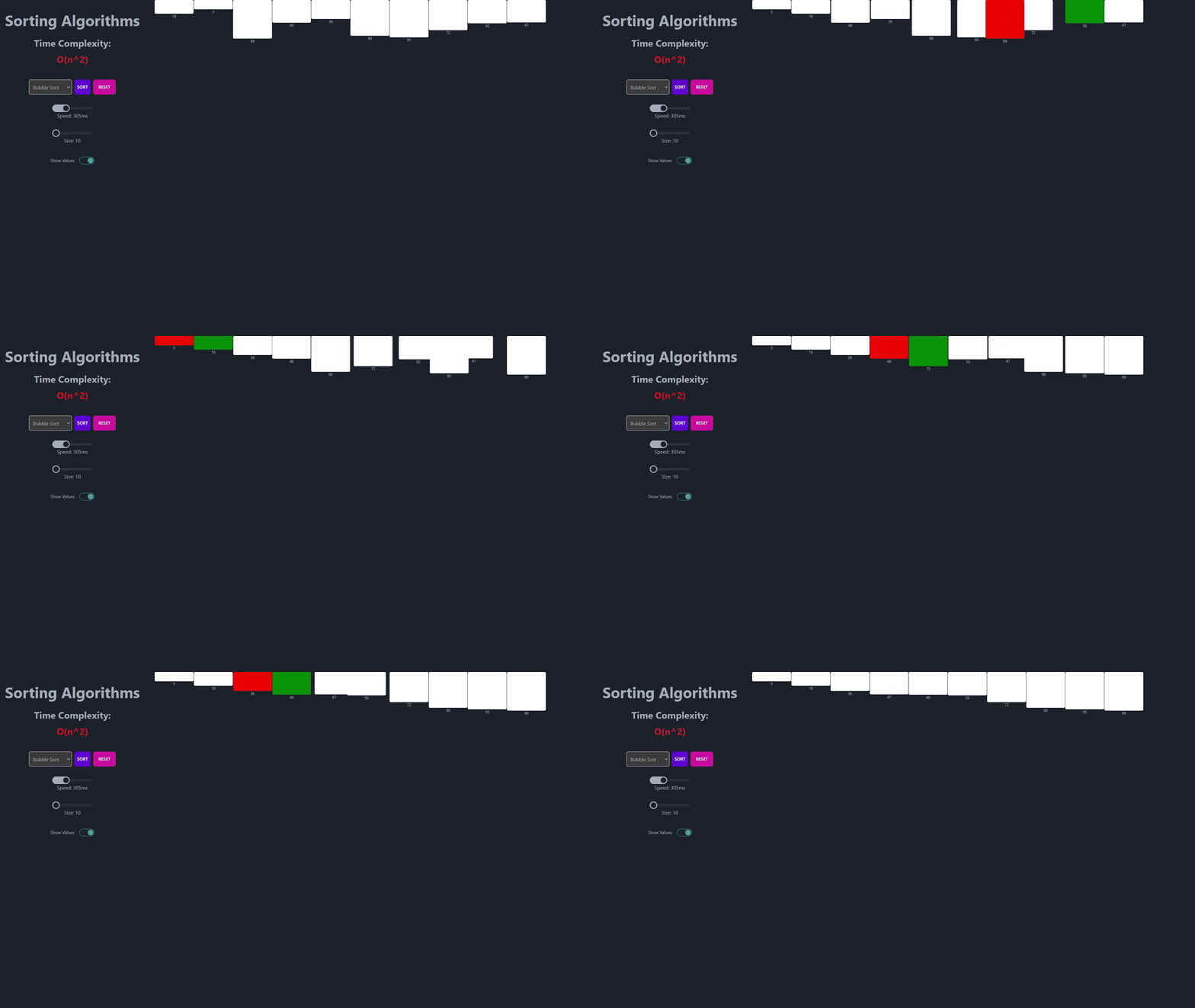
• Sorting Algorithms
  • Bubble Sort
  • Selection Sort
  • Insertion Sort
  • Merge Sort
  • Quick Sort
• Searching Algorithms
  • Linear Search
  • Binary Search
  • Jump Search
  • Exponential Search
• Maze Generation Algorithms
  • Binary Tree Algorithm
  • Randomized Backtracking (DFS)
  • Randomized Prim
  • Randomized Kruskal
  • Hunt and Kill
• Pathfinding Algorithms
  • Dijkstra's Algorithm
  • A* Search
  • Breadth-First Search
  • Depth-First Search
• Data Structures
  • Stack
  • Queue
  • Linked List
• Recommendation System
  • Collaborative Filtering
  • Content-Based Filtering

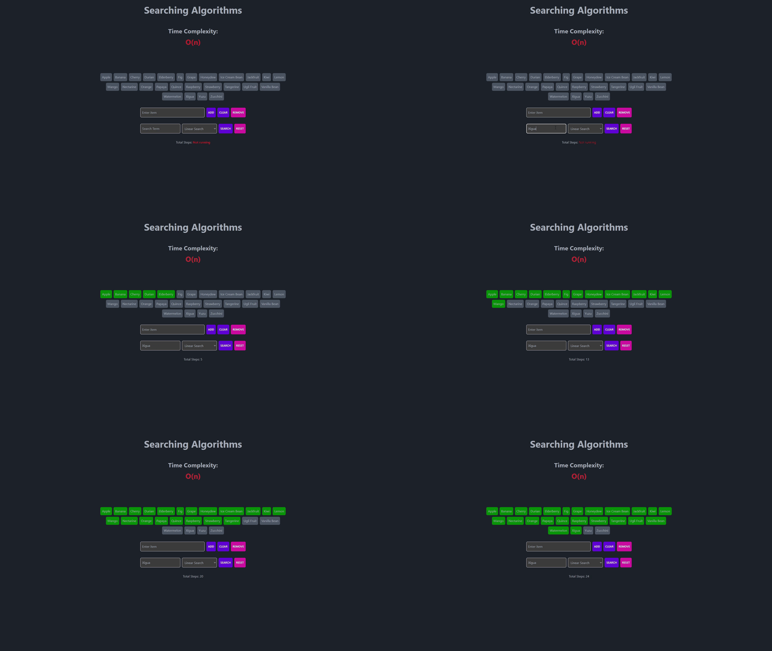
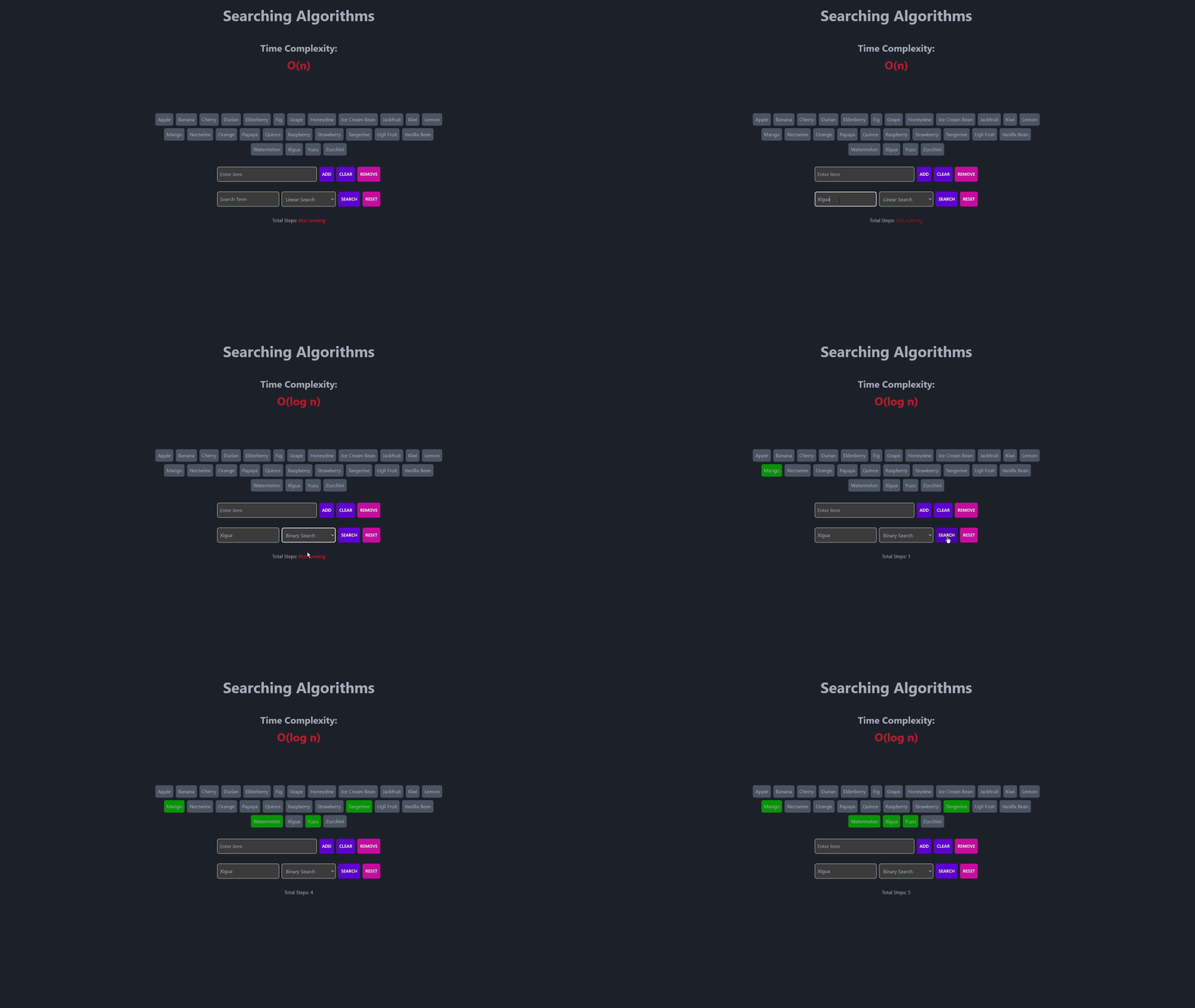
Sorting Algorithms

Mergesort and Quicksort have some minor issues with the visualization. I will fix them soon.

Bubble Sort

• This is the simplest sorting algorithm.
• It repeatedly compares adjacent elements and swaps them if they are in the wrong order.
• Time complexity is O(n²) in the worst case.
• Space complexity is O(1) in the worst case..

Selection Sort

• This algorithm sorts an array by repeatedly finding the minimum element from the unsorted part and putting it at the beginning.
• Time complexity is O(n²) in the worst case.
• Space complexity is O(1) in the worst case.

Insertion Sort

• This algorithm sorts an array by repeatedly inserting an element from the unsorted part into its correct position in the sorted part.
• Time complexity is O(n²) in the worst case.
• Space complexity is O(1) in the worst case.

Merge Sort

• This algorithm divides the array into two halves, sorts them separately, and then merges the two sorted halves.
• Time complexity is O(n log n) in the worst case.
• Space complexity is O(n) in the worst case.

Quick Sort

• This algorithm picks an element as a pivot and partitions the array around the pivot.
• Time complexity is O(n²) in the worst case.
• Space complexity is O(log n) in the worst case.

Searching Algorithms

Linear Search (Sequential Search)

• This is the simplest search algorithm.
• It sequentially checks each element in a list until a match is found.
• Works well for small lists or unsorted data.
• Time complexity is O(n) in the worst case.

Binary Search

• This is a more efficient search algorithm, but it requires sorted data.
• It repeatedly divides the search interval in half to find the desired item.
• Time complexity is O(log n) in the worst case.

Jump Search

• Jump Search divides the list into smaller blocks and checks these blocks to reduce the number of comparisons.
• Requires sorted data.
• Time complexity is O(√n) in the worst case.

Exponential Search

• Exponential Search finds the range in which the desired item is located by jumping 2ⁱ elements in every iteration and then performs a binary search in that range.
• Requires sorted data.
• Time complexity is O(log n) in the worst case.

Maze Generation Algorithms

Binary Tree Algorithm

• Complexity: Simplest
• This algorithm creates a maze by repeatedly carving passages either to the north or to the east.
• It is a simple algorithm, but it produces mazes with a strong north-east bias.
• It doesn't require maintaining a complex state or backtracking.

Randomized Backtracking (DFS)

• Complexity: Moderate
• Involves a stack and backtracking to create a maze
• It generates mazes with a single solution and a moderate level of complexity, but the paths tend to have a long and winding nature.

Randomized Prim

• Complexity: More Complex
• This algorithm creates a maze by randomly selecting a wall from the list of walls that separate cells in the maze and removing it if the cells on both sides of the wall belong to different sets.
• It's more efficient in space utilization than the DFS method.

Randomized Kruskal

• Complexity: Most Complex
• This algorithm creates a maze by randomly selecting a wall from the list of walls that separate cells in the maze and removing it if the cells on both sides of the wall belong to different sets.
• Produces mazes with a high degree of complexity and less bias compared to the other algorithms.

Hunt and Kill

• Complexity: A little more complex than DFS
• This algorithm creates a maze by randomly selecting a cell and carving a passage in a random direction from that cell.
• It then performs a random walk, carving passages to unvisited cells until it reaches a dead end.

Pathfinding Algorithms

Dijkstra's Algorithm

• This algorithm finds the shortest path between two nodes in a graph.
• It uses a priority queue to keep track of the next node to visit.

A* Search

• This algorithm is an extension of Dijkstra's algorithm.
• It uses a heuristic function to estimate the distance between the current node and the destination node.
• It uses a priority queue to keep track of the next node to visit.
• It is faster than Dijkstra's algorithm.

Breadth-First Search

• This algorithm finds the shortest path between two nodes in a graph.
• It uses a queue to keep track of the next node to visit.

Depth-First Search

• This algorithm finds the shortest path between two nodes in a graph.
• It uses a stack to keep track of the next node to visit.

Data Structures

Stack

• A stack is a linear data structure that follows the Last In First Out (LIFO) principle.
• It has two main operations: push and pop.
• It can be implemented using an array or a linked list.
• Time complexity of push and pop operations is O(1).
• Space complexity is O(n).

Queue

• A queue is a linear data structure that follows the First In First Out (FIFO) principle.
• It has two main operations: enqueue and dequeue.
• It can be implemented using an array or a linked list.
• Time complexity of enqueue and dequeue operations is O(1).
• Space complexity is O(n).

Linked List

• A linked list is a linear data structure that consists of nodes.
• Each node has a data field and a pointer to the next node.
• It can be implemented using a singly linked list or a doubly linked list.
• Time complexity of insertion and deletion operations is O(1).
• Space complexity is O(n).

Recommendation System

Collaborative Filtering

Will not be implemented

• This algorithm finds similar users based on their ratings and recommends items that they have rated highly.
• It uses the Pearson correlation coefficient to measure the similarity between users.
• It uses the weighted average of ratings to predict the ratings of items.

Content-Based Filtering

• This algorithm recommends items that are similar to the items that the user has liked in the past.
• It uses the cosine similarity to measure the similarity between items.
• It uses the weighted average of ratings to predict the ratings of items.

Planned work

1. Get images from unsplash
2. Use GCP Vision API to get labels

{
  "1.jpg": [
    {
      "locations": [],
      "properties": [],
      "mid": "/m/0c9ph5",
      "locale": "",
      "description": "Flower",
      "score": 0.9955990314483643,
      "confidence": 0,
      "topicality": 0.9955990314483643,
      "boundingPoly": null
    },
    {
      "locations": [],
      "properties": [],
      "mid": "/m/04sjm",
      "locale": "",
      "description": "Flowering plant",
      "score": 0.9854584336280823,
      "confidence": 0,
      "topicality": 0.9854584336280823,
      "boundingPoly": null
    },
    [...]
  ]
}

3. Format data
4. Calculate TF-IDF
5. Calculate cosine similarity between images
6. Use labels to find similar images
7. Use similar images to find similar items
8. Use similar items to recommend items