Overview:
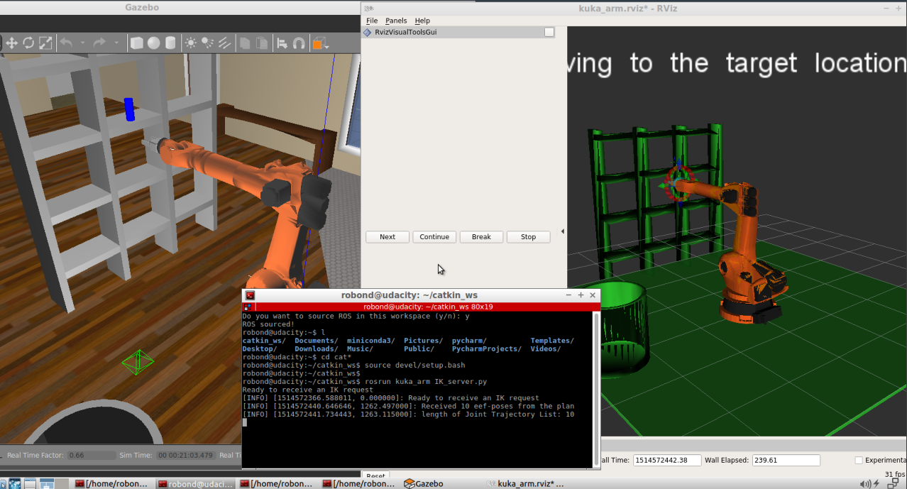
The target of this project is to provide a kinematic analisys for Kuka R210 robotic arm. In the simulation we process a task to pick, move and drop off an object into a box. In this project I will use ROS system and Gazebo + Rviz as simulation environment. Using Inverse Kinematic (IK), we can find the correct trajectory to drive the arm to drop the object in the desired place. The complete project can be found in this repository and here is the video.
Figure 1.
The kinematic analysis mainly includes two aspects, namely the forward kinematic analysis (FK) and the inverse kinematic analysis (IK). The forward kinematic analysis means that the pose of end-effector of Kuka can be worked out with the given geometry parameters of the links and the variables of the joints. Robots have either translational or rotational joints. A translational moves a point in space a finite distance along given vector direction, and it can be described by the following homogeneous transformation matrix between neighboring links, as showed in Fig. 2.
Figure 2.
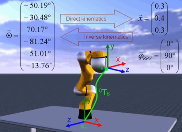
The solution for a forward kinematic (FK) problem is a straight calculation where we can use the joint angles and find the end-effector pose (position + orientation) of the robot arm. The Fig. 3 below shows the analysis model between FK and IK.
Figure 3.
But what is a link or a joint angle? We will see in the next section. The relashionship between links and joint angles of a robot can be derived using the Denavit-Hartenberg (DH) convention.
Reading the kr210.urdf.xacro file to perform kinematic analysis of Kuka KR210 robot and derive its DH parameters, resulting in Table 1 below.
Table 1.
| Links | alpha(i-1) | a(i-1) | d(i-1) | theta(i) |
|---|---|---|---|---|
| 0->1 | 0 | 0 | 0.75 | 0 |
| 1->2 | -pi/2 | 0.35 | 0 | -pi/2 + q2 |
| 2->3 | 0 | 1.25 | 0 | 0 |
| 3->4 | -pi/2 | -0.054 | 1.50 | 0 |
| 4->5 | pi/2 | 0 | 0 | 0 |
| 5->6 | -pi/2 | 0 | 0 | 0 |
| 6->EE | 0 | 0 | 0.303 | 0 |
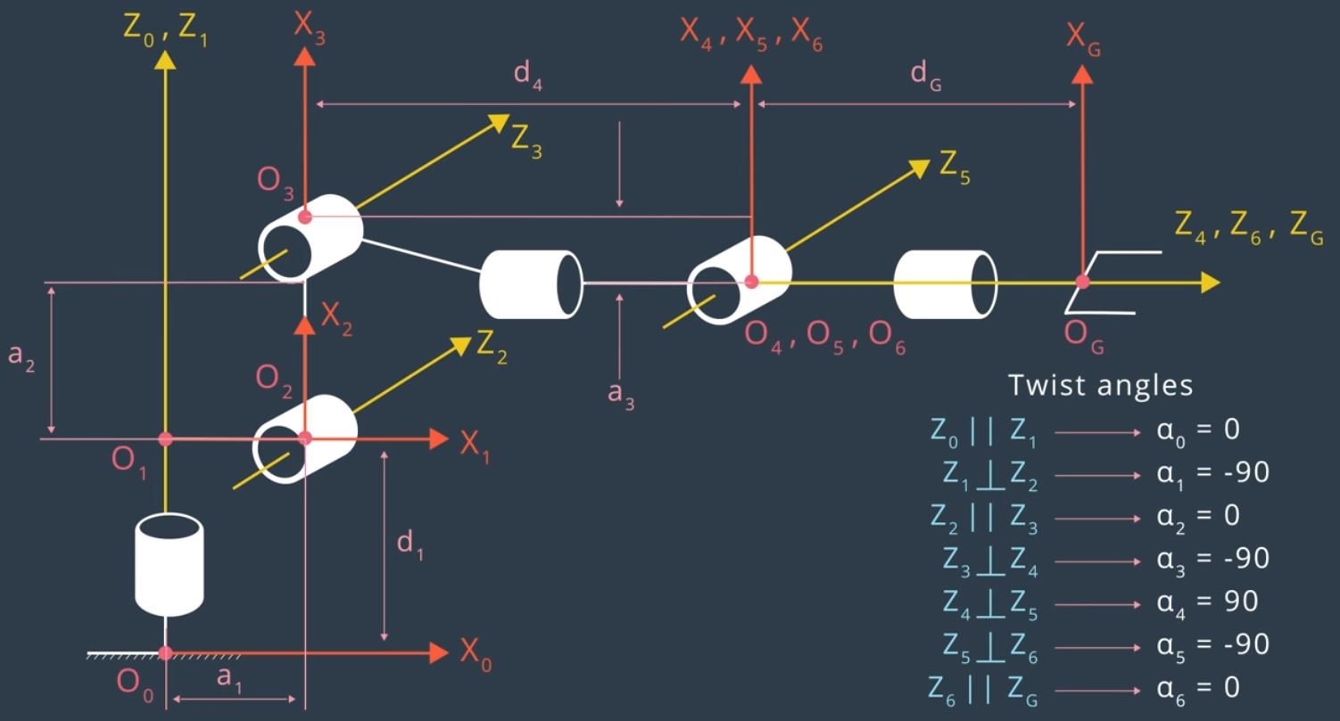
The DH parameters are given by the transformations from the coordinate system i-1 to i, via the rotational and translational transformations given in Table 1. Note that this is a modified convention from DH convention. The Fig. 4 shows the position of each variable described in Table 1.
Figure 4.
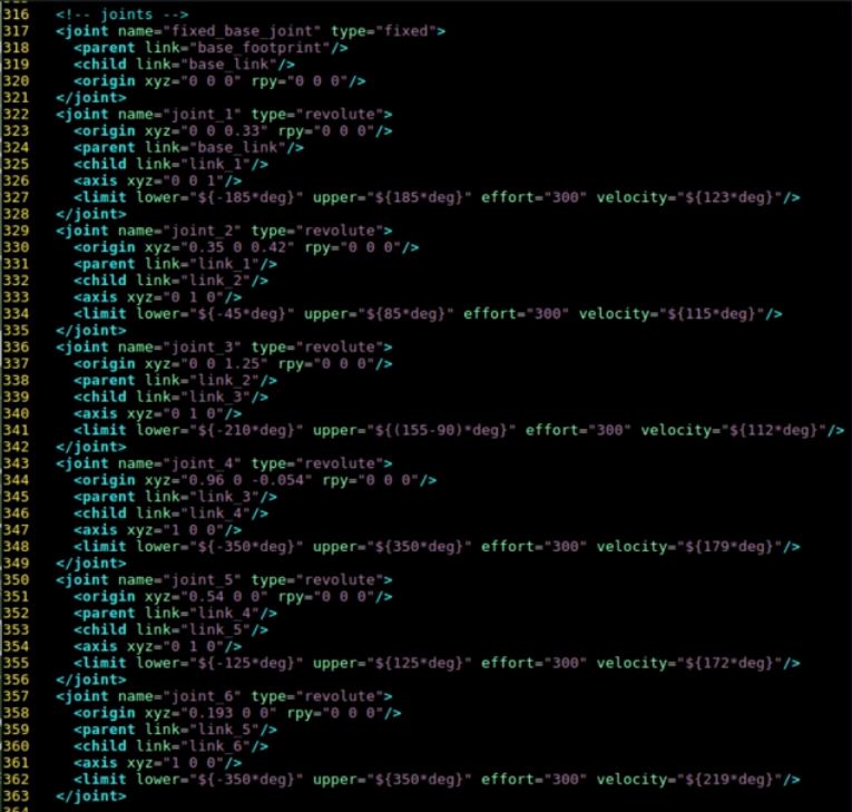
In Gazebo, the DH parameters table are described by a URDF file. All the joints and links are described in details in URDF file. The Fig. 5 below shows part of Kuka R210 URDF file.
Figure 5.
For instance, note that joint_3 is linked with the parent link_2 and the child link_3.
So, using the values in Table 1 and the homogeneous transformation formula described in Fig. 2, we can create the individual transformation matrices about each joint. In addition, we can also generate a generalized homogeneous transform between base_link and gripper_link using only end-effector (gripper) pose.
For instance, the homogeneous transform from base_link and link_1 (T0_1) can be written as follow:
def Tn_m(th, alpha, a, d):
    t = Matrix([[        cos(th),            -sin(th),            0,              a],
    [ sin(th)*cos(alpha), cos(th)*cos(alpha), -sin(alpha), -sin(alpha)*d],
    [ sin(th)*sin(alpha), cos(th)*sin(alpha),  cos(alpha),  cos(alpha)*d],
    [                   0,                   0,            0,               1]])
# Transformation from base_link to Link_1
T0_1 = Tn_m(q1, alpha0, a0, d1).subs(s)
And we repeat the same approach for all the others links
# Trasformation from link_1 to Link_2
T1_2 = Tn_m(q2, alpha1, a1, d2).subs(s)
# Transformation from link_2 to Link_3
T2_3 = Tn_m(q3, alpha2, a2, d3).subs(s)
# Transformation from link_3 to Link_4
T3_4 = Tn_m(q4, alpha3, a3, d4).subs(s)
# Transformation from link_4 to Link_5
T4_5 = Tn_m(q5, alpha4, a4, d5).subs(s)
# Transformation from link_5 to Link_6
T5_6 = Tn_m(q6, alpha5, a5, d6).subs(s)
# Transformation from link_6 to gripper G
T6_G = Tn_m(q7, alpha6, a6, d7).subs(s)
Then using the equations above, for each homogeneous transform from base_link to gripper_link, we have:
T0_1 = Matrix([ [cos(q1), -sin(q1), 0,    0],
                [sin(q1),  cos(q1), 0,    0],
                [      0,        0, 1, 0.75],
                [      0,        0, 0,    1]])

T1_2 = Matrix([[sin(q2),  cos(q2), 0, 0.35],
               [      0,        0, 1,    0],
               [cos(q2), -sin(q2), 0,    0],
               [      0,        0, 0,    1]])

T2_3 = Matrix([[cos(q3), -sin(q3), 0, 1.25],
               [sin(q3),  cos(q3), 0,    0],
               [      0,        0, 1,    0],
               [      0,        0, 0,    1]])

T3_4 = Matrix([ [ cos(q4), -sin(q4), 0, -0.054],
                [       0,        0, 1,    1.5],
                [-sin(q4), -cos(q4), 0,      0],
                [       0,        0, 0,      1]])

T4_5 = Matrix([ [cos(q5), -sin(q5),  0, 0],
                [      0,        0, -1, 0],
                [sin(q5),  cos(q5),  0, 0],
                [      0,        0,  0, 1]])

T5_6 = Matrix([ [ cos(q6), -sin(q6), 0, 0],
                [       0,        0, 1, 0],
                [-sin(q6), -cos(q6), 0, 0],
                [       0,        0, 0, 1]])

T6_G = Matrix([ [1, 0, 0,     0],
                [0, 1, 0,     0],
                [0, 0, 1, 0.303],
                [0, 0, 0,     1]])
And so, we can calculate the complete FK for the gripper pose.
Note that the homogeneous transform has a translational and a rotational section. Using this property we can rearrange the homogeneous transform and write the following:
Figure 6.
And it will result in the wrist center pose.
Inverse kinematic analysis is the opposite of forward kinematic analysis. Now the things are a bit more complex. Given a desired end-effector pose, we need find the values of the joint angles that will realize the correct trajectory to the target position. With the inverse kinematic solutions, the value of each joint angle can be determined in order to place the arm at a desired position and orientation.
That said, we need find the values of q1,q2,q3,q4,q5 and q6 that will move the arm to a desired pose.
Figure 7.
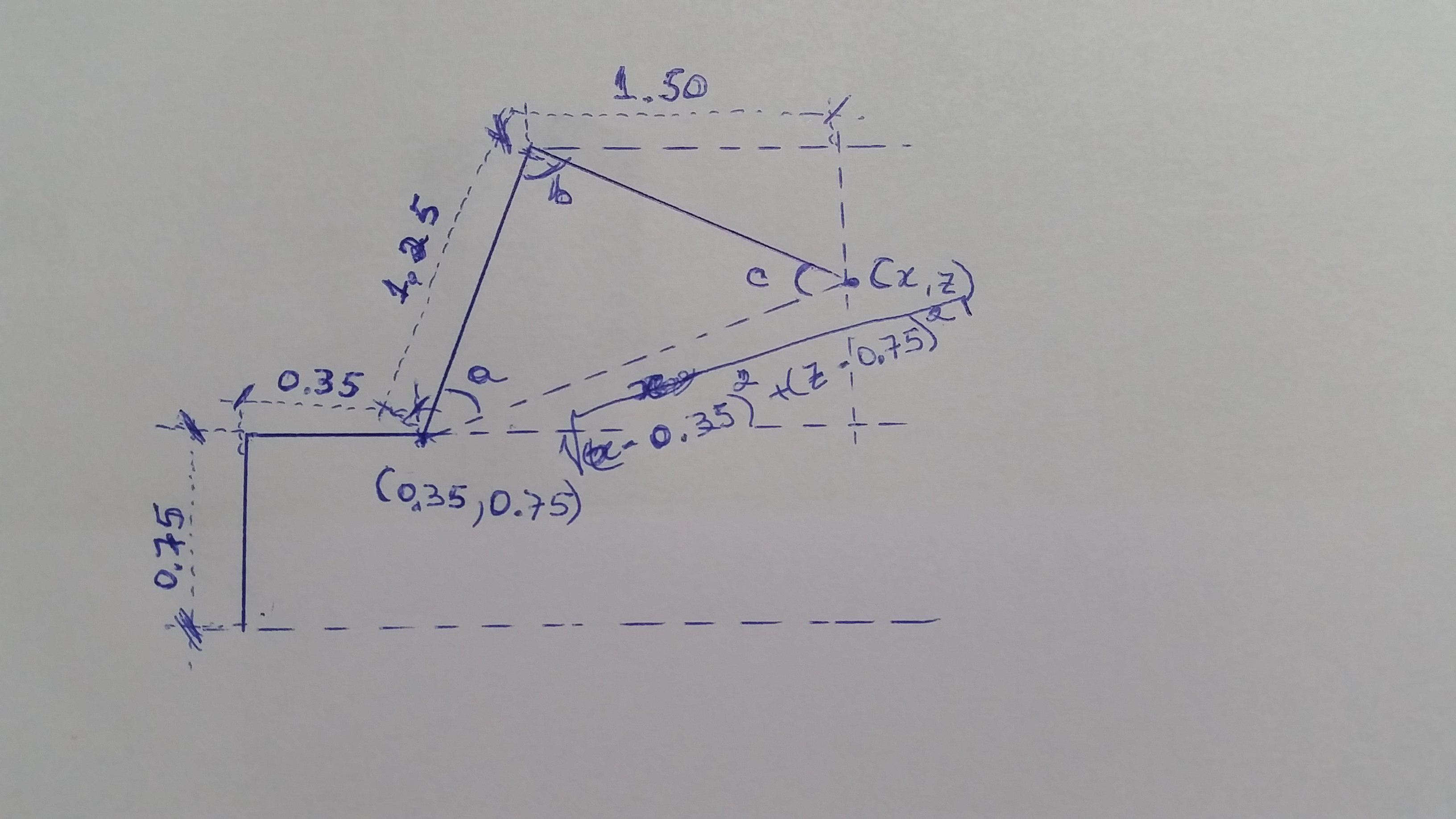
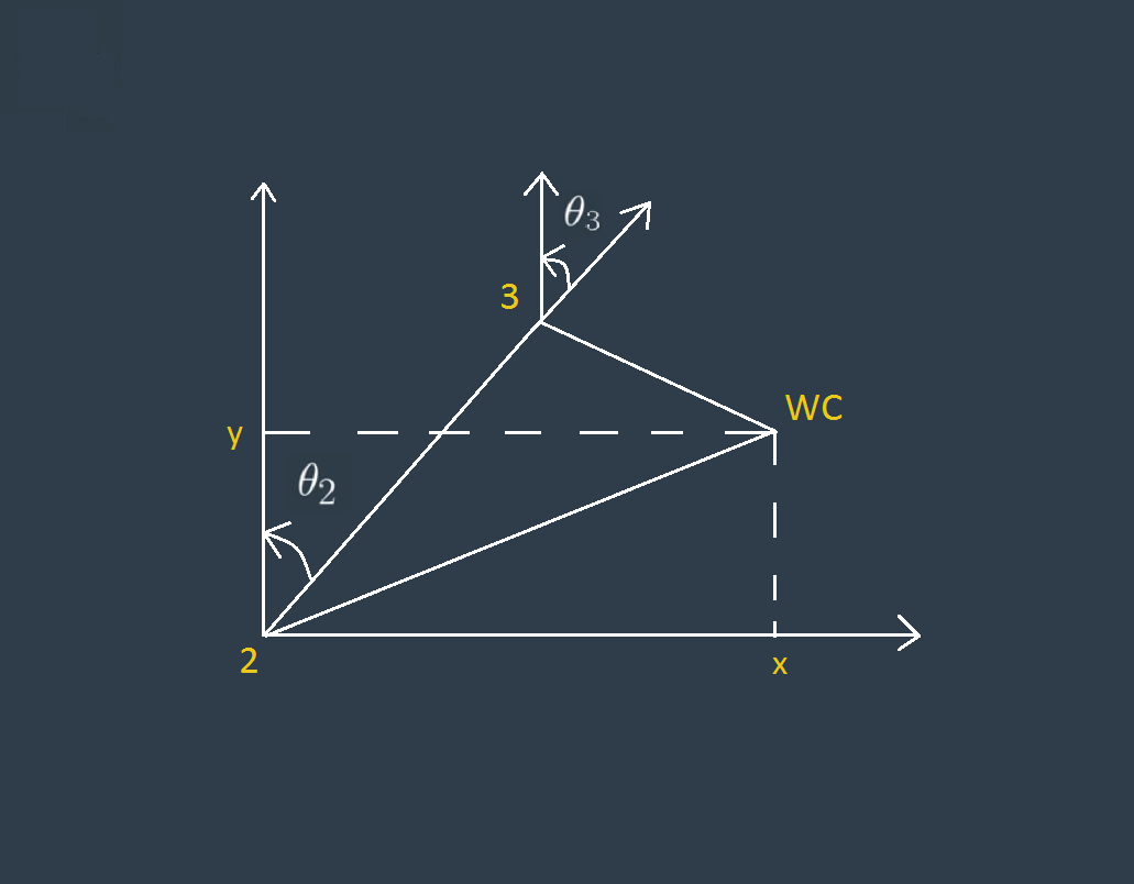
The values of q1,q2 and q3 are quite stright using some geometry properties of the arm as showed in Fig. 7
The q1 angle can be found from the projection of the arm over plane X0-Y0 and we get:
theta1 = atan2(Wc[1], Wc[0])The theta2 and theta3 we can get from Fig. 7 and Fig. 8 below.
Figure 8.
# using geometry to calculate the triangle sides
side_a = 1.501
side_b = sqrt(pow((sqrt(Wc[0] * Wc[0] + Wc[1] * Wc[1]) - 0.35), 2) + pow((Wc[2] - 0.75), 2))
side_c = 1.25
# using geometry to calculate the triangle angles
angle_a = acos((side_b * side_b + side_c * side_c - side_a * side_a) / (2 * side_b * side_c))
angle_b = acos((side_a * side_a + side_c * side_c - side_b * side_b) / (2 * side_a * side_c))
# calculate theta2
theta2 = np.pi / 2. - angle_a - atan2(Wc[2] - 0.75, sqrt(Wc[0] * Wc[0] + Wc[1] * Wc[1]) - 0.35)
# calculate theta3
theta3 = np.pi / 2. - (angle_b + 0.036)
Finally, using the rotation matrix R3_6 and more geometry properties, we can find the remaining angles q4, q5 and q6.
# Using rotational matrix to calculate remaining joint angles
# from transformation matrix we can extract the rotational matrix
R0_3 = oClass.T0_3[0:3, 0:3]
R0_3 = R0_3.evalf(subs={q1: theta1, q2: theta2, q3: theta3})
R3_6 = R0_3.T * Rot_G

# Now get Euler angles from rotation matrix
# calculate theta4
theta4 = atan2(R3_6[2, 2], -R3_6[0, 2])
# calculate theta5
theta5 = atan2(sqrt(R3_6[0, 2] * R3_6[0, 2] + R3_6[2, 2] * R3_6[2, 2]), R3_6[1, 2])
# calculate theta6
theta6 = atan2(-R3_6[1, 1], R3_6[1, 0])
# because this model has some singularities, we may consider
if( sin(theta5) < 0 ):
    theta4 = atan2(-R3_6[2, 2], R3_6[0, 2])
theta6 = atan2(R3_6[1, 1], -R3_6[1, 0])- Simulation environment: ROS running Gazebo + Rviz
- Languages: Python and C++
- OS: Ubuntu 16.04 running on VMware Pro
To run this project I implemented the code for FK and IK in the IK_server.py script file. The python code receives the end-effector pose, process the kinematics analysis and returns an array list with joint angles that will allow the arm to move to the new desired pose.
I had to optimize some issues with Kuka arm that was failing to pick the object. The IK was moving the arm correctly from start to end drop position but the process had no success because the gripper was failing to pick the object. Then I did two changes in the trajectory_sampler.cpp code:
- added 4 seconds before the gripper process function
- increased the gripper angle from 0.02 to 0.025
Then these two changes decreased the probabilities to gripper fail to keep the object.
Another challenge was find a solution to avoid run the symbolic code inside the loop that manage the received poses from the arm. The calculation of symbolic variables takes a long time, mainly because we have many matrix operations. So, consider, for instance, 60 sec to complete the symbolic operations and then multiply by 50, 60, 100 poses iterations and you will get a big computational time. At final this would be an unacepptable time for each cycle.
To fix this issue I created a class to manage the creation of all symbolic variables and calculations. Then I executed that class code once, creating an object that was serialized and saved to disk. So, in the project I IK_server.py code just need to load (deserialize) the object. This approach takes only fractions of seconds which means a fast computational time in the loop that manage FK and IK analysis.
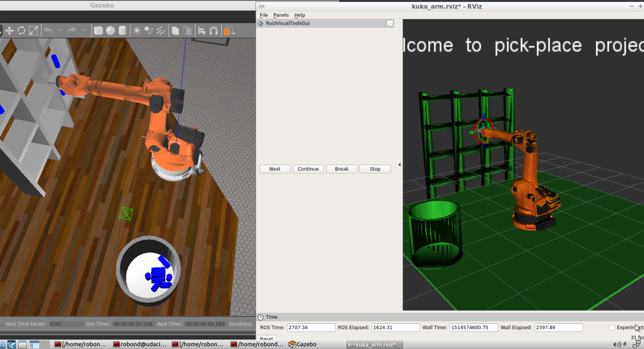
Figure 9.
The Fig, 9 shows the final process after 10 tries. Note that there are 3 pins in the boxes and 8 in the dropbox. One is for cycle 11 and must not be considered. But the others 2 are in the boxes because, even the gripper pose was correct, it failed to keep the object in the gripper.
So, we can conclude that the errors in FK and IK calculations are very low and if we had a better gripper operation, we could achieve 100% in 10 tries.
Improve the gripper operation to avoid fail pick the object even when the gripper is in the correct pose.
