stefmolin / ml-utils

Machine learning utility functions and classes.

Machine learning utility functions and classes

All examples derived from chapters 9-11 in my book, Hands-On Data Analysis with Pandas (1st edition, 2nd edition).

Note: This package uses scikit-learn for metrics calculation; however, with the except of the PartialFitPipeline the functionality should work for other purposes provided the input data is in the proper format.

Setup

# should install requirements.txt packages
$ pip install -e ml-utils # path to top level where setup.py is

# if not, install them explicitly
$ pip install -r requirements.txt

Example Usage

Classification

Plot a confusion matrix as a heatmap:

>>> from ml_utils.classification import confusion_matrix_visual
>>> confusion_matrix_visual(y_test, preds, ['white', 'red'])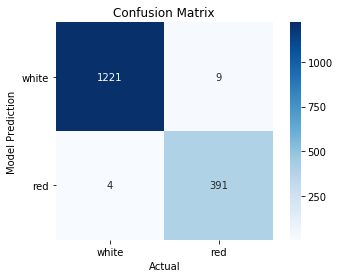

ROC curves for binary classification can be visualized as follows:

>>> from ml_utils.classification import plot_roc
>>> plot_roc(y_test, white_or_red.predict_proba(X_test)[:,1])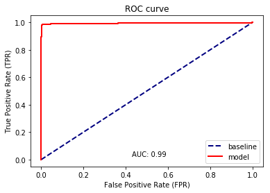

Use ml_utils.classification.plot_multi_class_roc() for a multi-class ROC curve.

Precision-recall curves for binary classification can be visualized as follows:

>>> from ml_utils.classification import plot_pr_curve
>>> plot_pr_curve(y_test, white_or_red.predict_proba(X_test)[:,1])

Use ml_utils.classification.plot_multi_class_pr_curve() for a multi-class precision-recall curve.

Finding probability thresholds that yield target TPR/FPR:

>>> from ml_utils.classification import find_threshold_roc
>>> find_threshold_roc(
...     y_jan, model.predict_proba(X_jan)[:,1], fpr_below=0.05, tpr_above=0.75
... ).max()
0.011191747078992526

Finding probability thresholds that yield target precision/recall:

>>> from ml_utils.classification import find_threshold_pr
>>> find_threshold_pr(
...     y_jan, model.predict_proba(X_jan)[:,1], min_precision=0.95, min_recall=0.75
... ).max()
0.011191747078992526

Elbow Point Plot

Use the elbow point method to find good value for k when using k-means clustering:

>>> from sklearn.pipeline import Pipeline
>>> from sklearn.preprocessing import StandardScaler
>>> from ml_utils.elbow_point import elbow_point

>>> elbow_point(
...     kmeans_data, # features that will be passed to fit() method of the pipeline
...     Pipeline([
...         ('scale', StandardScaler()), ('kmeans', KMeans(random_state=0))
...     ])
... )

Pipeline with partial_fit()

>>> from sklearn.linear_model import SGDClassifier
>>> from sklearn.preprocessing import StandardScaler
>>> from ml_utils.partial_fit_pipeline import PartialFitPipeline

>>> model = PartialFitPipeline([
...     ('scale', StandardScaler()),
...     ('sgd', SGDClassifier(
...         random_state=0, max_iter=1000, tol=1e-3, loss='log',
...         average=1000, learning_rate='adaptive', eta0=0.01
...     ))
... ]).fit(X_2018, y_2018)

>>> model.partial_fit(X_2019, y_2019)
PartialFitPipeline(memory=None, steps=[
    ('scale', StandardScaler(copy=True, with_mean=True, with_std=True)),
    ('sgd', SGDClassifier(
       alpha=0.0001, average=1000, class_weight=None,
       early_stopping=False, epsilon=0.1, eta0=0.01, fit_intercept=True,
       l1_ratio=0.15, learning_rate='adaptive', loss='log', max_iter=1000,
       n_iter=None, n_iter_no_change=5, n_jobs=None, penalty='l2',
       power_t=0.5, random_state=0, shuffle=True, tol=0.001,
       validation_fraction=0.1, verbose=0, warm_start=False
    ))
])

PCA

Use PCA with two components to see if the classification problem is linearly separable:

>>> from ml_utils.pca import pca_scatter
>>> pca_scatter(wine_X, wine_y, 'wine is red?')
>>> plt.title('Wine Kind PCA (2 components)')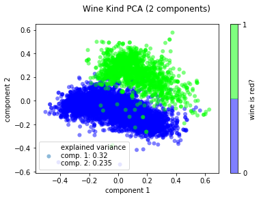

Try in 3D:

>>> from ml_utils.pca import pca_scatter_3d
>>> pca_scatter_3d(wine_X, wine_y, 'wine is red?', elev=20, azim=-10)
>>> plt.title('Wine Type PCA (3 components)')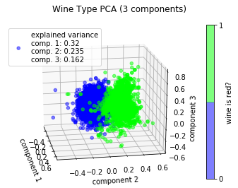

See how much variance is explained by PCA components, cumulatively:

>>> from sklearn.decomposition import PCA
>>> from sklearn.pipeline import Pipeline
>>> from sklearn.preprocessing import MinMaxScaler
>>> from ml_utils.pca import pca_explained_variance_plot

>>> pipeline = Pipeline([
...     ('normalize', MinMaxScaler()), ('pca', PCA(8, random_state=0))
... ]).fit(X_train, y_train)

>>> pca_explained_variance_plot(pipeline.named_steps['pca'])

See how much variance each PCA component explains:

>>> from sklearn.decomposition import PCA
>>> from sklearn.pipeline import Pipeline
>>> from sklearn.preprocessing import MinMaxScaler
>>> from ml_utils.pca import pca_scree_plot

>>> pipeline = Pipeline([
...     ('normalize', MinMaxScaler()), ('pca', PCA(8, random_state=0))
... ]).fit(w_X_train, w_y_train)

>>> pca_scree_plot(pipeline.named_steps['pca'])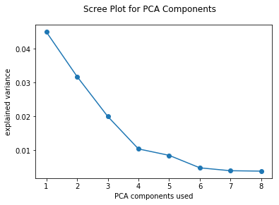

Regression

With the test y values and the predicted y values, we can look at the residuals:

>>> from ml_utils.regression import plot_residuals
>>> plot_residuals(y_test, preds)

Look at the adjusted R^2 of the linear regression model, lm:

>>> from ml_utils.regression import adjusted_r2
>>> adjusted_r2(lm, X_test, y_test)
0.9289371493826968

---

About the Author

Stefanie Molin (@stefmolin) is a software engineer and data scientist at Bloomberg in New York City, where she tackles tough problems in information security, particularly those revolving around data wrangling/visualization, building tools for gathering data, and knowledge sharing. She is also the author of Hands-On Data Analysis with Pandas, which is currently in its second edition and has been translated into Korean. She holds a bachelor’s of science degree in operations research from Columbia University's Fu Foundation School of Engineering and Applied Science, as well as a master’s degree in computer science, with a specialization in machine learning, from Georgia Tech. In her free time, she enjoys traveling the world, inventing new recipes, and learning new languages spoken among both people and computers.