sohonisaurabh / CarND-Kidnapped-Vehicle-Project

This repository contains C++ code for implementation of Particle Filter to localize a vehicle kidnapped in a closed environment. This task was implemented to partially fulfill Term-II goals of Udacity's self driving car nanodegree program.

CarND-Kidnapped-Vehicle-Project

This repository contains C++ code for implementation of Particle Filter to localize a vehicle kidnapped in a closed environment. This task was implemented to partially fulfill Term-II goals of Udacity's self driving car nanodegree program.

Background

A critical module in the working of a self driving vehicle is the localizer or localization module. Localization can be defined as predicting the location of vehicle with high accuracy in the range 3-10 cm. This location is in reference to a global map of the locality in which the self driving vehicle is either stationery or moving.

One way to localize a vehicle is by using data from Global Positioning System (GPS), which makes use of triangulation to predict the position of an object detected by multiple satellites. But GPS doesn't always provide high accuracy data. For e.g.: In case of strong GPS signal, the accuracy in location is in the range of 1-3 m. Whereas in the case of a weak GPS signal, the accuracy drops to a range of 10-50 m. Hence the use of only GPS is not reliable and desirable.

To achieve an accuracy of 3-10 cm, sensor information from Laser sensor (LIDAR) and/or Radial distance and angle sensor (RADAR) is used and fused together using a Particle Filter. This process is demonstrated in the following sections.

Localization Algorithm

Localization in case of self driving vehicle makes use of GPS, range sensors, landmark information and a global map based on the following algorithm given below:

1. A global map of different areas is constructed, in which the self driving vehicle is to be deployed. This map contains information about different location of 'landmarks'. Landmarks are nothing but major features present in the locality, which are not subject to change for a longer period of time. Examples can be buildings, signal posts, intersections, etc. These landmarks are used in later steps to predict the relative location of car. These maps are updated often so as to add new features and refresh the locations of existing features.

2. Once a map is constructed, GPS sensor installed inside the vehicle is used to predict the locality in which it is present. On basis of this locality, only a portion of global map is selected to avoid a large number of real time calculations as the algorithms must run in real time. As stated earlier, GPS sensor provides noisy measurement and hence cannot be used alone for localization.

3. LIDAR and/or RADAR sensor installed on the vehicle then measure the distance between it and the landmarks around it. This helps in further pinning down location of the vehicle as it is now relative to landmarks in the global map constructed earlier. However, LIDAR and RADAR information is also not accurate and prone to noise. Hence, a sophisticated technique like Particle Filter is used.

4. Particle Filter is used to combine the information gained from all above steps and predict the location of car with high accuracy of 3-10 cm.

The whole algorithm repeats at run time when the car is moving and new location of car is predicted.

Project Goal

In this project, a vehicle is kidnapped inside a closed environment and has no idea of its location. This environment is simulated in Udacity's self driving car simulator. The vehicle travels through the environment and takes roughly 2400 steps with change in orientation and position. The goal is to predict the location of vehicle using Particle Filter program implemented in C++. The error between ground truth location of robot and the predicted location should be minimal. Also, the program must be performant enough to run within 100 seconds while maintaining minimal error.

Project Implementation

Each major step involved in implementation is illustrated below:

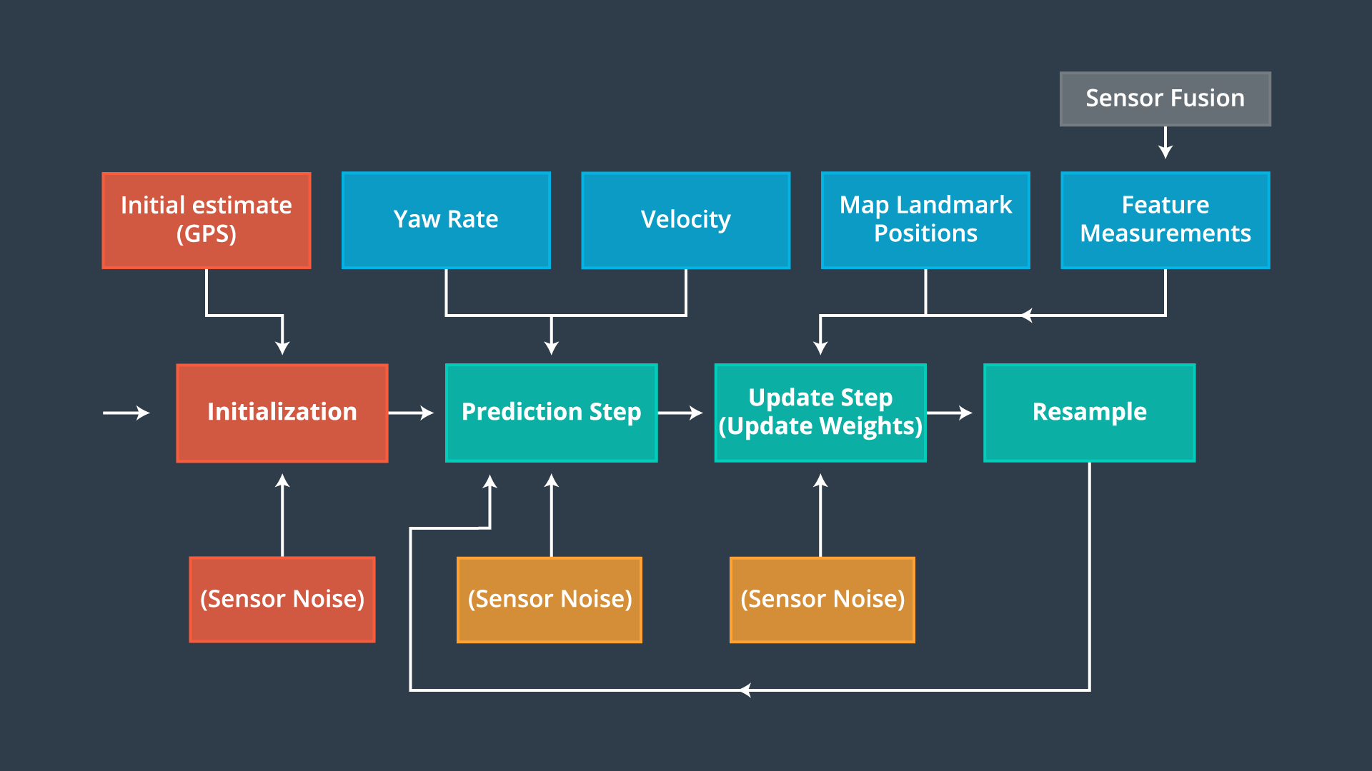
The C++ program for localization was implemented using following major steps:

1. A noisy measurement from GPS sensor was received and used to initialize the position of vehicle. This measurement included the x coordinate, y coordinate (both in m) and the theta (orientation) of vehicle in radian. Noise is modelled by Gaussian distribution with standard deviation in x, y and theta provided as a part of GPS uncertainty specification. Particle filter algorithm uses particles to represent the location of vehicle. Hence, in this case, 20 particles were created and initialized to locations taken from normal distribution with mean equal to the location received from GPS and standard deviation equal to the GPS measurement uncertainty. The number of particles was a tunable parameter and was chosen after multiple iterations described in later steps of implementation.

2. Global map of environment is initialized. This map is represented by a list x and y coordinates of landmarks in the environment.

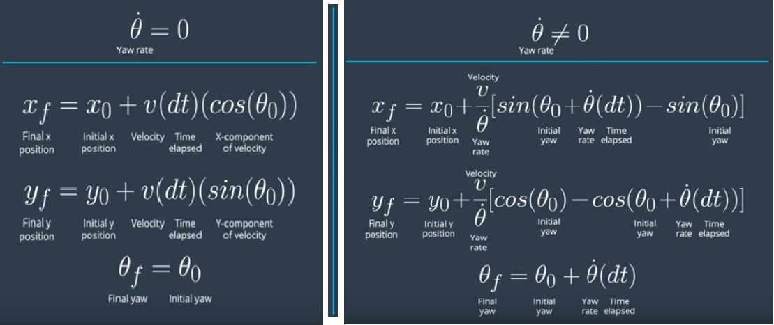
3. Once map and particles are initialized, the vehicle implements Prediction step in which the location of each particle at next time step is predicted. This is done by using information of control inputs and time elapsed between time steps. The control inputs are nothing but magnitude of velocity (v) and yaw rate (θ). Location update is done with the help of formula given below:

4. After prediction step, the vehicle implements Update step. In this step, particles are assigned with weights corresponding to their prediction. The process is stated below:

a. The vehicle uses LIDAR to sense its distance from landmarks and predict the location of landmarks as observed. This is received as a list of x, y coordinates along with the noise mapped as standard deviation in X (σx) and Y (σy) axes. Since, the LIDAR sensor is installed on the robot, these observations are received in x, y coordinate axes relative to the direction of motion of vehicle. This is shown below:

Here, X axis is in the direction of motion of the vehicle and Y axis is perpendicular to X axis to the left.

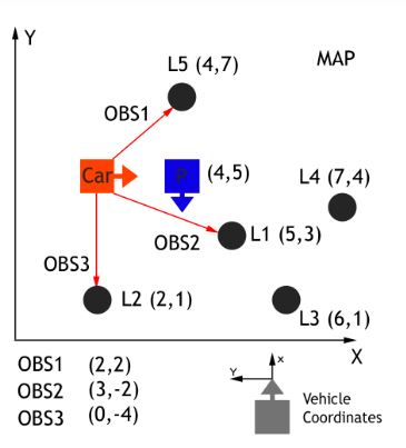
The landmarks are shown with annotations L1-L5. Observations recorded in vehicle's coordinates are annotated OBS1-OBS3. The ground truth of vehicle is shown in red while the prediction of location vehicle as derived by the particle is shown in blue.

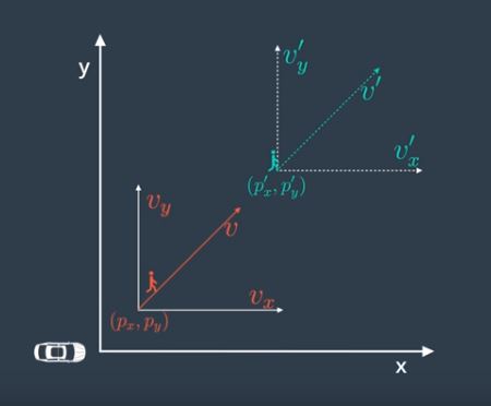
b. To map the observations into global coordinate system, a transformation is done involving translation and rotation but no scaling. This is done by using Homogenous Coordinate Transformation given by the formula below:

where xm, ym represent the transformed observation, xc, yc represent the observations in vehicle's coordinate system and xp, yp the location of particle in global map coordinate system.

c. All landmarks cannot be in the range of vehicle at a given point of time. This is determined by the range of LIDAR sensor. Hence, given the observations at a time, all probable landmarks in the range of a particle are determined. This step involves filtering of landmarks to retain only those which are in the range of the particle.

d. After landmarks are filtered, each observation is then mapped to a landmark using nearest neighbor algorithm. The nearest neighbor algorithm is implemented by calculating Euclidean distance between an observation and all landmarks. The landmark with lowest Euclidean distance is associated to the observation. Hence, multiple observations may be associated to a single landmark.

e. Once every observation is associated to a landmark, weight of the particle is calculated by using Multivariate Gaussian distribution. Since all observations are independent, the total weight of the particle is the product of probabilities calculated by Multivariate Gaussian formula for all observations associated to landmarks. Formula for calculation of individual probabilities is given below:

where x and y is the observation and µx and µy are the coordinates of associated landmark. The final weight of particle is product of all probabilities.

f. The weight of particle is the measure of how close the particle is w.r.t. to the ground truth of vehicle. The higher the weight, the more accurate is the particle's prediction. Hence, at the end of each update step, 'resampling' of particles with replacement is done to remove highly improbable particles.

The update step is (a-f) is run for every particle and weight of each particle is calculated.

6. After udapte, resampling of particles is done. Resampling involves retaining of particles with higher weight and crushing of particles with lower weight. Once resampling is done, the particle with highest weight is chosen. This particle gives most accurate prediction of vehicle's location.

7. The location provided by particle with highest weight is then compared with the ground truth and error in the system is calculated.

8. Once initialization, prediction, update and resampling is implemented, the program is run under testing and error in the system along with run time is noted. To get the best estimate of vehicle's position in real time, the number of particles is tuned and finalized.

Project Output

Particle filter implemented was run on Udacity's simulator and its error and performance was noted. Below are the results with 10 and 20 particles respectively:

Run 1: 10 particles

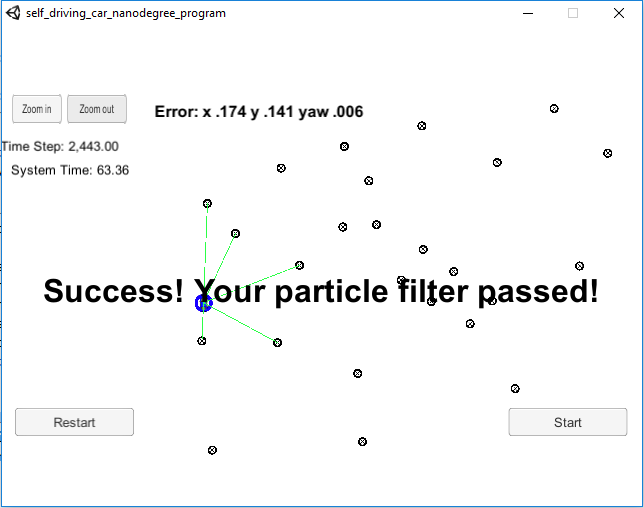
Run 2: 20 particles

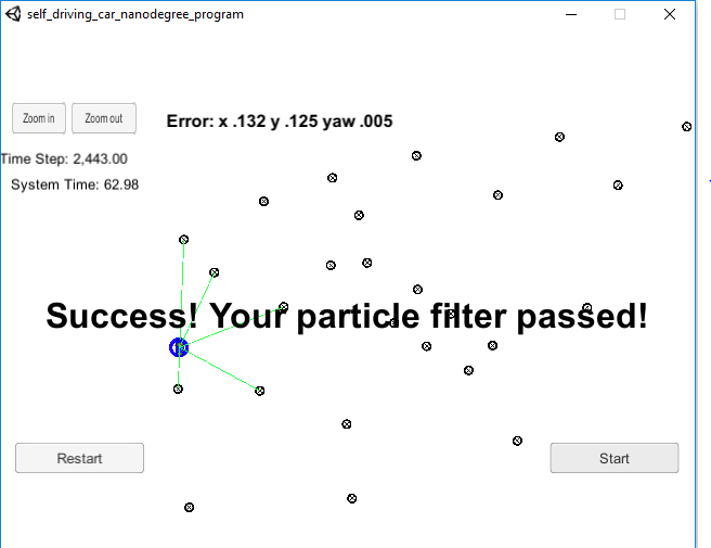
In both the runs, implementation was declared as pass since the error and the execution time of code was in permissible limits.

Steps for building the project

Dependencies

• cmake >= 3.5

• All OSes: click here for installation instructions

• Linux and Mac OS, you can also skip to installation of uWebSockets as it installs it as a dependency.

• make >= 4.1(mac, linux), 3.81(Windows)

  • Linux: make is installed by default on most Linux distros
  • Mac: install Xcode command line tools to get make
  • Windows: Click here for installation instructions
  • Linux and Mac OS, you can also skip to installation of uWebSockets as it installs it as a dependency.

• gcc/g++ >= 5.4

  • Linux: gcc / g++ is installed by default on most Linux distros
  • Mac: same deal as make - [install Xcode command line tools]((https://developer.apple.com/xcode/features/)
  • Windows: recommend using MinGW
  • Linux and Mac OS, you can also skip to installation of uWebSockets as it installs it as a dependency.

• uWebSockets

  • Run either install-mac.sh or install-ubuntu.sh. This will install cmake, make gcc/g++ too.
  • If you install from source, checkout to commit e94b6e1, i.e.

    git clone https://github.com/uWebSockets/uWebSockets 
    cd uWebSockets
    git checkout e94b6e1
    

    Some function signatures have changed in v0.14.x.

• Simulator. You can download these from the Udacity simulator releases tab.

Running the project in Ubuntu

1. Execute every step from ./install-ubuntu.sh. This will install gcc, g++, cmake, make and uWebsocketIO API.

2. Build and run project by running ./build.sh.

3. In case of error, manually build the project and run using: a. mkdir build && cd build b. cmake .. c. make d. ./particle_filter

4. Run the Udacity simulator and check the results