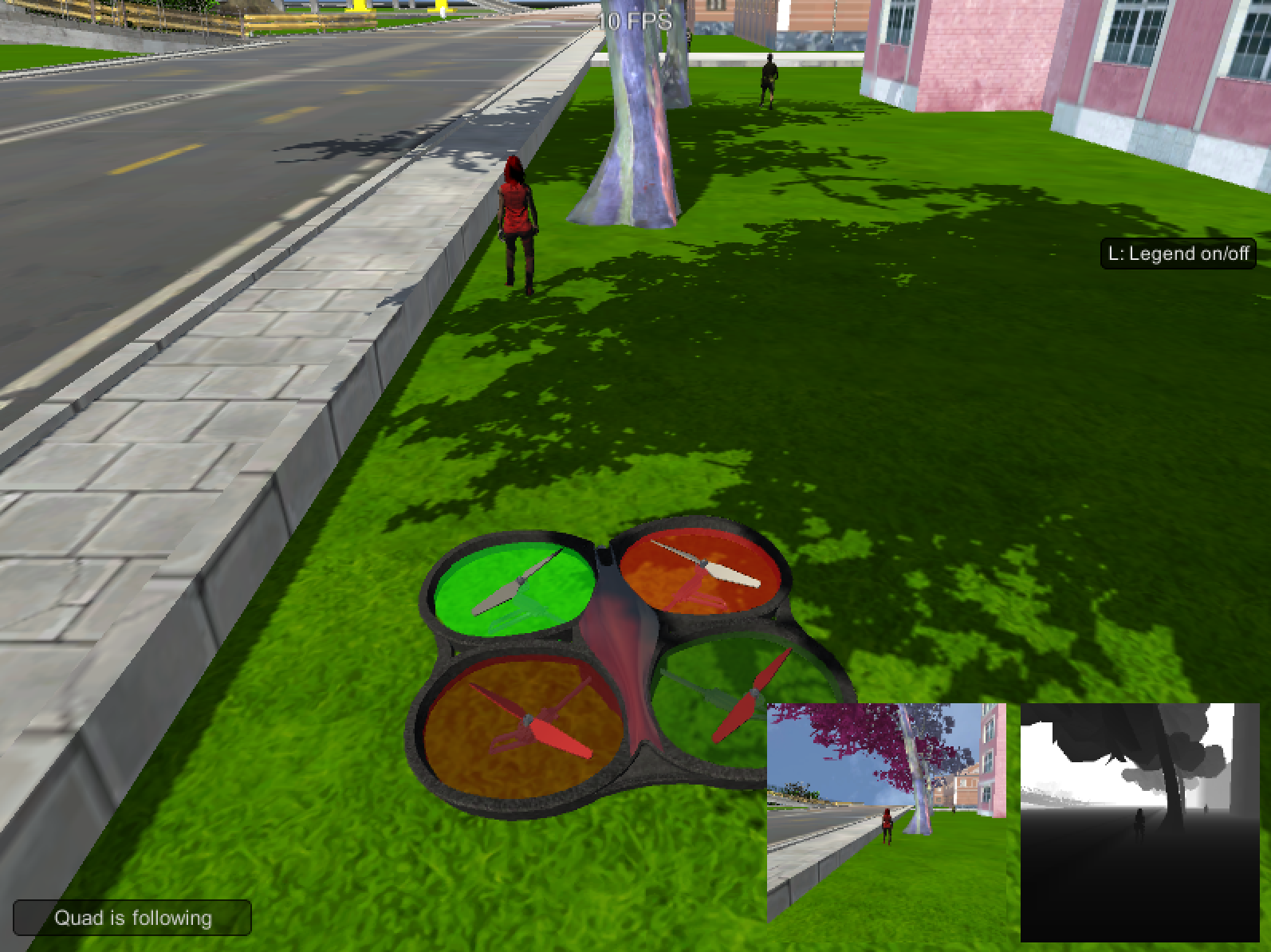
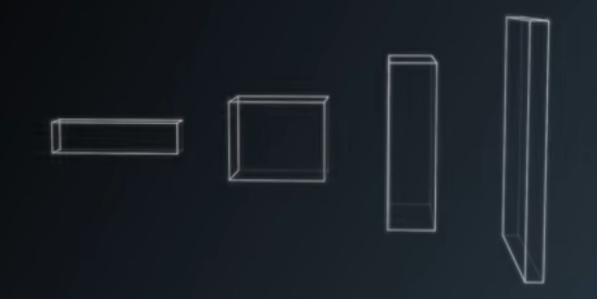
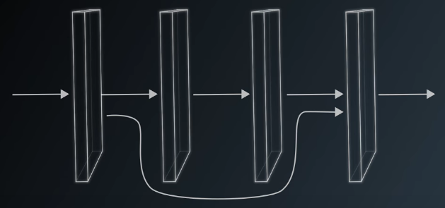
In this project, a deep neural network has been trained to identify and track a target in simulation. So-called “follow me” applications like this are key to many fields of robotics and the very same techniques we apply here can be extended to scenarios like advanced cruise control in autonomous vehicles or human-robot collaboration in industry.
Clone this repository.
Download the QuadSim binary
Download the simulator here
Install Dependencies
Use the environment.yml file in this repository.
conda env create -f environment.yml
Note: The following network has been trained on an Nvidia GTX 1060 3GB GPU. if you want to reproduce this project, you need a GPU with equal or more memory or you can run into "Resource Exhaust Error". Please see the /code/model_training.ipynb notebook in the code folder.
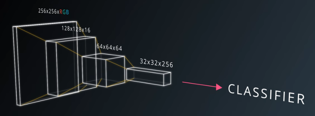
Convolution Neural Networks (covnets) have achieved state of the art in the image classification. A typical covnet would apply convolution filters over a shallow image and increase the depth while it squeezes the spatial dimensions. It starts with learning smaller features in the starting layers and as the depth increases, it can learn more complex features, objects shapes for instance. A few fully connected layers then can serve as a classfier. In addition, a covnet can make use of pooling and regulizers such as dropout.
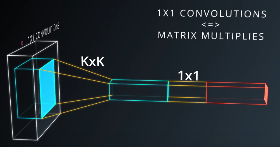
Covnets however can not tell where an object is in the image as the fully connected layers do not retain the spatial information. Some object detection models such as Yolo and SSD do a great job of object detection but can not classify each and every pixel in the image. Fully Convolution Networks come into play here (offcourse at the cost of computational complexity), where 1x1 convolution layer replaces a flattened layer, fully connected layers are replaced by transposed convolutional layers of increasing spatial dimensions and skip connections (making use of higher resolution information in the network). This helps classifying each pixel in the image by retaining spatial information throughout the network.
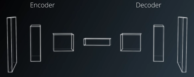
The Encoder part of the FCN extracts the features from the input image while Decoder upscales the image such that it is the same size as the input hence resulting in the classification of each pixel in the original image.
1x1 Convolution(4D tensor) replacing the flattened layer(2D tensor) of the covnet saves us from losing the spatial information in the image.
Transposed Convolutions or deconvolutions is simply the reverse of a simple convolution where forward and backward passes are swapped hence trainable in the same way. It helps upscaling the previous layer.
Downsampled convolutions lose some information and even upsampling to original image dimensions won't bring back the lost information. Skip connections work by adding or concatenating higher resolution layers from the encoder to the layers of same spatial dimensions in the decoder. Therefore the network can learn to make more accurate segmentation decisions.
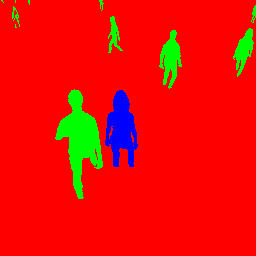
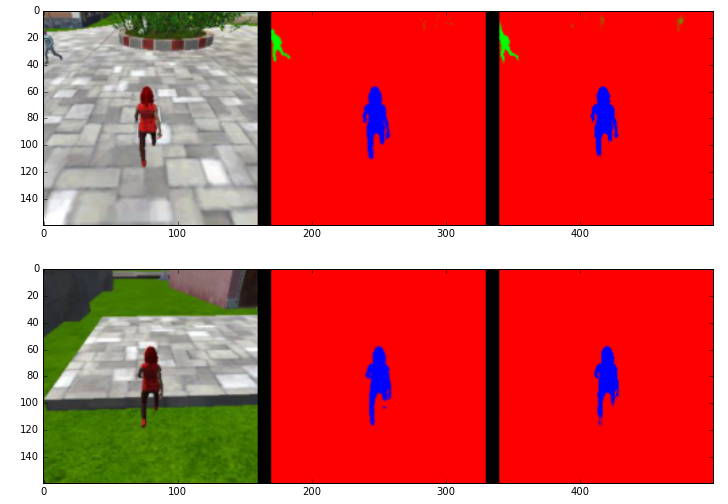
The goal here is to create an FCN architecture that segments an image into 3 classes; the target person, other people and the background.
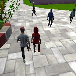
From the image above (160x160x3) for example, below is the labeled image with blue target, green other people and red background.
Now I'll dive straight into the network architecture. Please note that I'll discuss my best FCN architectire first. As discussed in the background, we need an encoder with convolution layers downsampling while increasing the depth of the image.
Since we want to use our model for real time inference, we have used Separable Convolutions also known as depthwise separable convolutions, instead of simple convolution. These comprise of a convolutions performed over each channel of an input layer and followed by a 1x1 convolution that takes the output channels from the previous step and then combines them into an output layer. This results in the reduction of the number of parameters therefore, quite efficient with improved runtime performance. They also have the added benefit of reducing overfitting to an extent, because of the fewer parameters.
Next is keeping our weights in the network within a certain range 0,1 for example with 0.5 mean and a standard deviation of 0.5. The reason behind normalizing our weights is that we have a huge loss function and we don't want our weights to explode or get too small; the optimizer would have a hard time optimizing otherwise. Instead of only normalizing our inputs to the network, here we use batch normalization after each layer in the network. It seems to have an added computational complexity, that's true, but later we can use a higher learning rate hence faster training. It also adds some noise hence acting as a good regulizer.
We also need normal convolution function for 1x1 convolutions with a kernel size of 1 and a stride of 1.
Next, we define our Encoder Block, which makes use of the alternating separable convolutions and the batch normalization. The encoder block is flexible and there are certain choices to be made, like filter depths of separable convolutions, kernel sizes, stride etc. I have stacked up two alternating separable convolutions/normalization where both convolutions have an equal number of filters and strides. Stacking up 2 alternating separable convolutions increase trainable parameters.
Now we can use the above created smaller encoder block to create our entire Encoder for the network. I have used 3 smaller encoder blocks:
- The first with the filter depths of 64 and a stride of 1 hence resulting in the output tensor of [None, 160, 160, 64]. The reason I haven't downsampled the input yet is that I want to use this first smaller encoder output as a skip connection (as it has the best high level information about the image). It could have been done with original input but during experimentation, using input layer as a skip connection to the output layer introduced noise, therefore applying filters straight away and not downsampling helped retained useful information. I also tried varying depths of 16, 32 but the more number of filters, the more there are trainable parameters resulting in better results. Further increase in the filters would cause the GPU to run into memory issue.
- The next encoder has a depth of 256. Because of the stride of 2 applied to both inside separable convolutions, there is a sudden downsampling to size [None, 40, 40, 256], therefore the filter depth sizes lower than 256 would result in considerable loss of information. And increasing depth further risks memory exhaustion. I use this layer as a second skip connection to the second last layer of the network.
- The last encoder again uses a stride of 2, resulting in [None, 10, 10, 1024] tensor. Since the spatial dimensions have been sqeezed too much, the filter depth is increased 4 times again resulting in [None, 10, 10, 1024]. I didn't use this layer as a skip connection ahead because doing so in earlier experiments increased the weights a lot and didn't bring better results because of extremely reduced spatial dimensions.
This completes the encoder block and a 1x1 convolution can be applied, I have used a depth of 4096 for 1x1 convolutions i.e. [None, 10, 10, 4096].
Now before I move to the decoder part, it would be nice to have a network diagram:
Oops, the architecture looks too big here. That's because of using multiple alternating convolutions/normalizations in both the encoder and decoder blocks and then multiple instances of these. Next we need to upsample the 1x1 convolutional layer to the original image size.
Earlier we mentioned the transposed convolution, but here we use the bilinear upsampling which is more efficient because it utilizes the weighted average of four nearest known pixels, located diagonally to a given pixel, to estimate a new pixel intensity value. The weighted average is usually distance dependent. The bilinear upsampling method does not contribute as a learnable layer like the transposed convolutions in the architecture and is prone to lose some finer details, but it helps speed up performance.
Next I have defined two blocks, a decoder block and a simpler upsampling block. Both use bilinear upsampling but the decoder block has an additional concatenation block with helps adding the skip connections from the previous layers. And just like the encoder block, these have 2 alternating convolution/batch normalization layers with equal number of filters again increasing the trainable parameters.
To complete our entire decoder block, we use the following:
- A simple upsampling block with filter depths of 512 and results in [None, 20, 20, 512] tensor.
- A decoder block with filter depths of 256 and concatenating the output of the second smaller encoder block hence [None, 40, 40, 256] tensor. Note here that this decoder has reduced the depth of concatenated layer fron 768 to 256. (See model summary in /code/model_training.ipynb or /code/model_training.html)
- An upsampler again so that the next decoder may have the same spatial dimensions as the first smaller encoder block. This upsampler resutls in [None, 80, 80, 64].
- Another decoder with 16 filters, upsizes to [None, 160, 160, 64], concatenates with the first smaller encoder to [None, 160, 160, 128] applies two alternating separables/normalizations with filter to [None, 160, 160, 16].
And finally we have an output layer with 3 channels and a softmax activation to have our logits. We can now proceed to training the network.
I have used the Udacity provided data only, but for an even better model, more data can be collected by running the simulator in the training mode.
I have used the following hyperparameters to train the network.
learning_rate = 0.001 batch_size = 8 num_epochs = 100 steps_per_epoch = 200 validation_steps = 50 workers = 2
With the batch normalization layers in place, we can set a higher learning rate of 0.001. A rate of 0.0001 is too slow and would need a lots of epochs to train (A rough intuition is > 200) where one epoch can take anywhere from 60 seconds to 140 seconds depending upon the architecture (not reducing spatial dimensions abrubptly gave me a run of around 128 seconds). A batch size of 16 would very often cause me run into memory issues on a 3GB GPU (Smaller architectures run fine but no better performance). Hence I have used a batch size of 8 to have maximum flexibility for experimenting with varying architectures. However, with this small batch size, the learning rate can not be increased further because it would cause weight biasness with every batch, which may be representing only one class at a time (only the background). The number of epochs I have chosen is certainly larger and for this particular scenario, 70 epochs would do a fine job only decreasing the end performance to 2-3%.
To train the network we use "categorical crossentropy" as our loss function and "Adam" optimizer. After training for 100 epochs, the network achieved a training loss of 0.0084 and validation loss of 0.0211. Because of lower batch size the validation loss sees spikes throughout the training process.
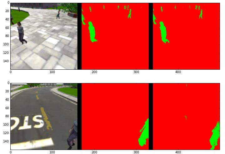
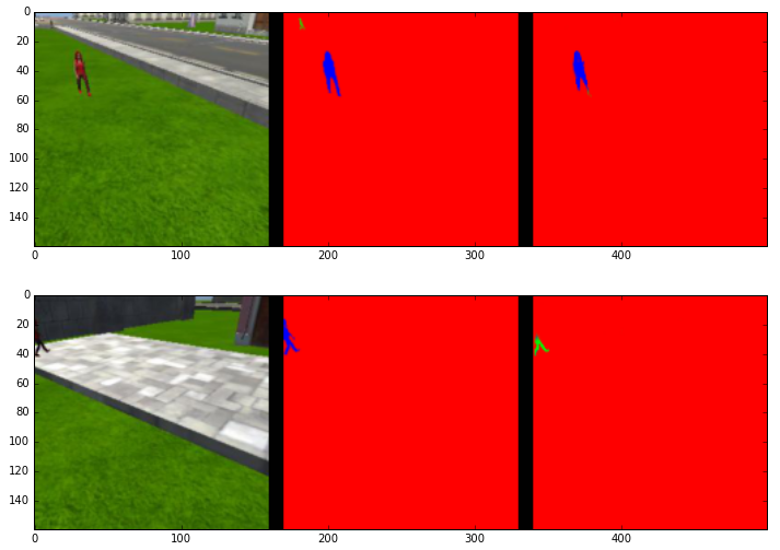
Now that we have our model trained and saved, we can make predictions on our validation dataset. These predictions can be compared to the mask images, which are the ground truth labels, to evaluate how well our model is doing under different conditions.
There are three different predictions available from the helper code provided:
Images while following the target
Images while at patrol without target
Images while at patrol with target at distance
To score the network on the Follow Me task, two types of error are measured. First the intersection over the union for the pixelwise classifications is computed for the target channel.
In addition to this we determine whether the network detected the target person or not. If more then 3 pixels have probability greater then 0.5 of being the target person then this counts as the network guessing the target is in the image.
We determine whether the target is actually in the image by whether there are more then 3 pixels containing the target in the label mask.
Using the above the number of detection true_positives, false positives, false negatives are counted.
How the Final score is Calculated
The final score is the pixelwise average_IoU*(n_true_positive/(n_true_positive+n_false_positive+n_false_negative)) on data similar to that provided in sample_evaulation_data. With this network architecture and the hyperparameters the final grade score was 48.5 which is an ok score without additional data and limited GPU memory.
Ideas for Improving Score
Collecting more data with target at medium and far distances will certainly improve the performance as we have lesser such samples. With a larger available memory, more encoding and decoding layers can be introduced with increased depth filters, hence more trainable parameters. A larger batch size would definitely bring better training results with fewer epochs. However, the key to Semantic Segmentation is the labeled data. This model would only work for detecting a target person with dominant red color dress or an object of similar shape. And no it can't detect cars, cats etc unless we have the available labeled data for such objects, but may be it can sometimes detect cars, dogs etc if they are red and network might misclassify these as target.
There are two more architectures which were able to achive the final grade score > 0.40. Since the write up is longer I have added only the html versions of those runs in the /code folder.
The network in file named model_training_40.9%.html achieves a score of 0.409. Within the smaller encoder block, it doubles the filters for second separable convolution and stride is 1 for first layer whereas variable for second layer. The upsampling and decoder blocks also use two seperable/normalization layers but the filters get halved for 2nd layer. 5 encoder, 2 upsampling and 2 decoder blocks are used with two skip connections. The details can be seen in the file.
In model_training_44.1.html however, I used single separable/normalization for encoder and decoder. However I have used 7 encoder and 3 decoder blocks with 3 skip connections. It scored 0.441.
Please note that the hyperparameters are the same for all the three architectures here.
