Advanced Lane Finding Project

The goals / steps of this project are the following:

Compute the camera calibration matrix and distortion coefficients given a set of chessboard images.
Apply a distortion correction to raw images.
Use color transforms, gradients, etc., to create a thresholded binary image.
Apply a perspective transform to rectify binary image ("birds-eye view").
Detect lane pixels and fit to find the lane boundary.
Determine the curvature of the lane and vehicle position with respect to center.
Warp the detected lane boundaries back onto the original image.
Output visual display of the lane boundaries and numerical estimation of lane curvature and vehicle position.

Usage

Calibration

python calibrate.py -o camera.p images

Produces camera matrix and distortion coefficients using given images set. Optionally one could pass optional parameter -g to produces samples of undistorted images.

Video Pipeline

python video.py -o output.mp4 input.mp4 -b 0 -e 42

Processes input video by applying the pipeline. Optional parameters -b and -e controls begin and end time of the clip.

Here's a link to my video result

Project Structure

averager.py - averager
calibrate.py - camera calibration utility
camera.py - routines to load/store camera parameters
cv_utils.py - various cv helpers/wrappers
fit.py - polynomial fit algorithm
fit_policy.py - fitting algorithm selector
mpp.py - real world conversion routines
perspective.py - functions related to warp perspective
pipeline.py - image processing pipeline
threshold.py - functions related to thresholding (both color and gradients)
video.py - video conversion utility

Camera Calibration

The code for this step is contained in calibration.py:66.

I start by preparing "object points" template (PATTERN_POINTS), which will be the (x, y, z) coordinates of the chessboard corners in the world. Here I am assuming the chessboard is fixed on the (x, y) plane at z=0, such that the object points are the same for each calibration image. Thus, object_points is just a replicated array of coordinates, and object_points will be appended with a copy for each successfully processed input image ( calibration.py:get_object_points()).

image_points will be appended with the (x, y) pixel position of each of the corners in the image plane with each successful chessboard detection. Additionally all images where chessboard detection failed were reported (calibration.py:get_image_points()) and used as a test images to control quality of calibration.

I then used object_points and image_points from all images (except one) where chessboard was detected successfully to compute the camera calibration matrix and distortion coefficients using the cv2.calibrateCamera() function.

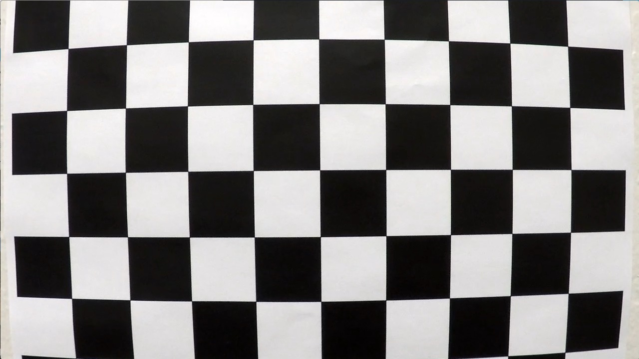
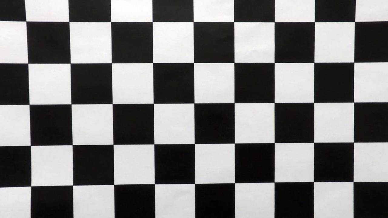
I applied this distortion correction to the test image using the cv2.undistort() function and obtained this result:

Pipeline (single images)

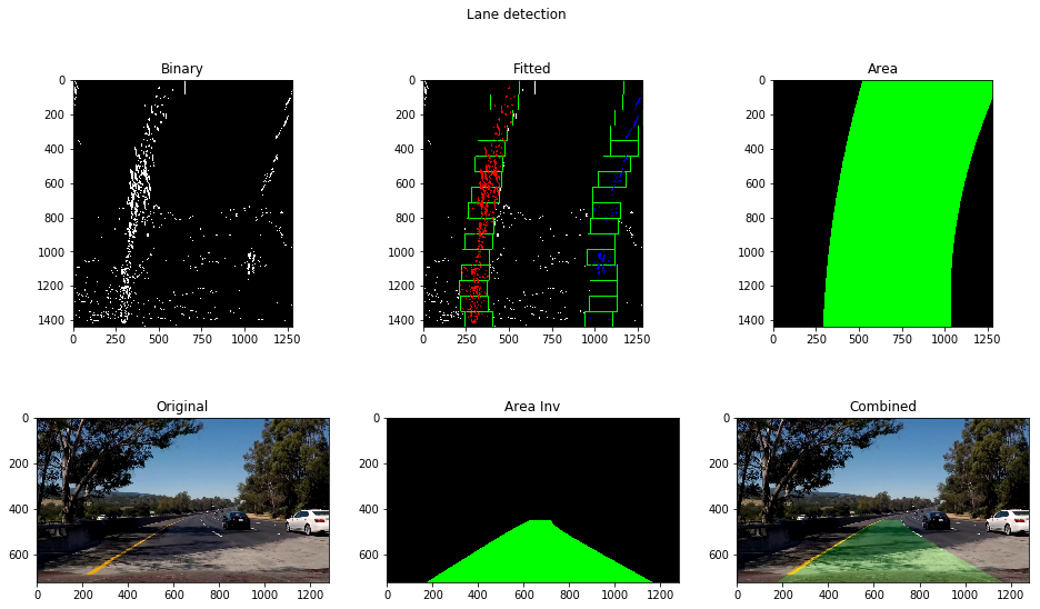
In the project I used the following image processing pipeline (detailed description could be found in pipeline.py:apply()):

Distortion correction
Warp perspective - I found it's useful to perform perspective transformation before any other (adjustments, thresholding) transformations, because after this transformation image contains only area of interest which increases overall efficiency of the pipeline
Some adjustments in image brightness and contrast
Thresholding
- Color thresholding
- Gradients thresholding
- Combination
Lane detection
Inverse warp perspective
Combination of original undistorted image and detected lane
Image annotation

Distortion-corrected image

To demonstrate this step, I will describe how I apply the distortion correction to one of the test images like this one.

This step as simple as applying cv2.undistort() routine with previously detected camera matrix and distortion coefficients.

Perspective transform

The code for my perspective transform includes a couple of functions called forward() and backward(). Which appears in lines 39 through 47 in the file perspective.py. Both functions take as inputs an image (image) and uses pre-calculated matrixes to perform transformation. The only difference for those functions is destination image size calculations.
I chose the hardcode the source and destination points in the following manner:

SCALE = 0.75 # used to narrow the lane a bit and make it easy to fit bigger curves

TD = 37 # top delta
TXR = 10 # top extra delta for the right lane
BD = 379 # bottom delta
BXR = 146 # bottom extra delta for the right lane

half_x = shape[1]//2
top, bottom = get_road_borders()

src = np.array([
        [half_x - TD, top],
        [half_x + TD + TXR, top],
        [half_x + BD + BXR, shape[0]],
        [half_x - BD, shape[0]],
    ], dtype=np.float32)

dst = np.array([
        [half_x - BD*SCALE, 0],
        [half_x + (BD + BXR)*SCALE, 0],
        [half_x + (BD + BXR)*SCALE, 2*shape[0]],
        [half_x - BD*SCALE, 2*shape[0]],
    ], dtype=np.float32)

This resulted in the following source and destination points:

Source	Destination
603, 450	356, 0
687, 450	1034, 0
1165, 720	1034, 1440
261, 720	356, 1440

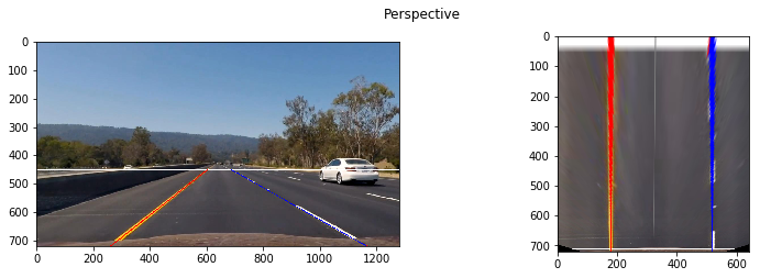
I verified that my perspective transform was working as expected by drawing the left and right lane lines onto a test image and verify that the lines appear parallel in the warped image.

Image Adjustment

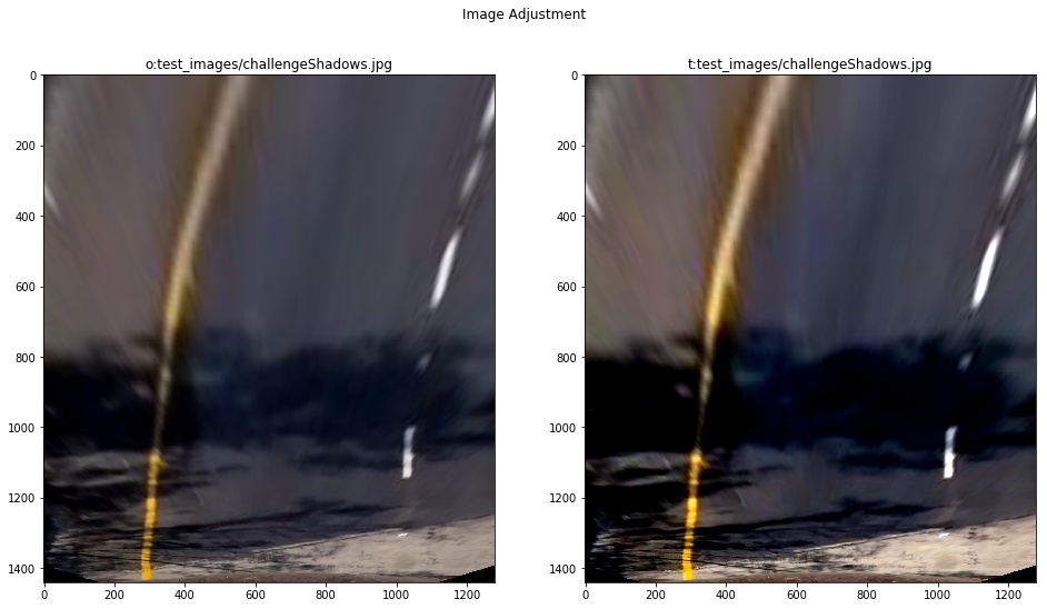
I used brightness and contrast adjustments on warped image in order to make further detection easier. The contrast was increased and brightness decreased. Exact parameters could be found in file pipeline.py as ADJUST_CONTRAST_FACTOR and ADJUST_BRIGHTNESS. The algorithm - cv_utils.py:adjust_image().

Thresholding

I used combination of color and gradients thresholds in the project. Functions responsible for creating binary image located in threshold.py. Functions take RGB and HLS images as an input. This was done intentionally - to avoid multiple HLS conversions, to experiment with more potential layers. Conversion between RGB and HLS color spaces was made using cv2.cvtColor function. See below for detailed description of used threshold algorithms.

Color thresholding

I used combination of hue and saturation thresholds of HLS color space to produce final binary mask for color thresholding step.
I applied threshold function on hue and saturation channels. Results was bitwise or-ed in order to produce final mask. Algorithm located in threshold.py:color_threshold().

Gradient thresholding

The main working horse of gradient thresholds - Sobel operator. In the project I used combination of 2 different Sobel operators. The implementation could be found in threshold.py:sobel_threshold()

The first set is - absolute x-coordinate value and direction thresholds on luminance channel of HLS image.

The second set is - full gradient magnitude and direction thresholds on saturation channel of HLS image.

The final binary images is bitwise or-ed of above two.

Combined thresholding

Finally previously defined binary images were bitwise or-ed in order to produce the final binary images for further process. The function defined in threshold.py:combined_threshold()

Lane Detection

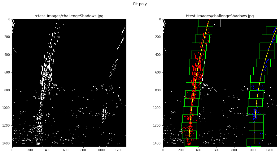
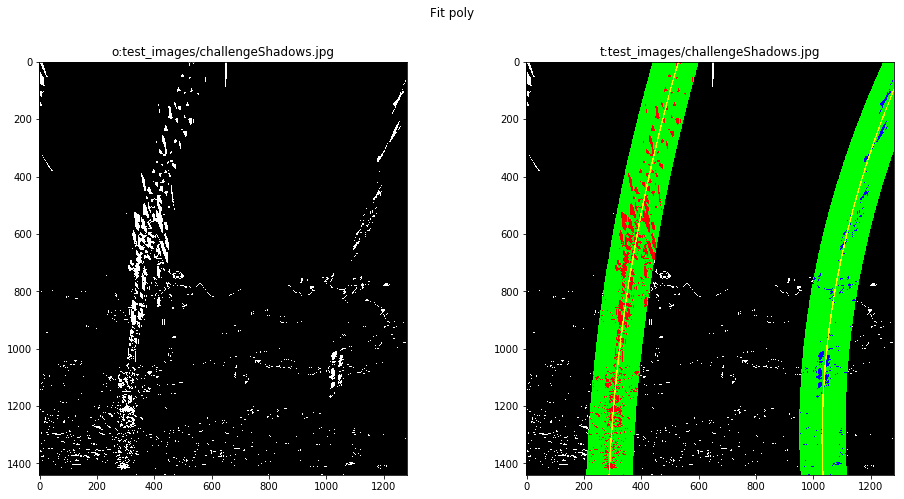
I used a variation of an algorithm described in the theory block. Basically there are 3 cases to identify lane-like pixels on the image and fit 2nd degree polynomial.

Blind search - using simple sliding window algorithm. Acceptance criteria - always
Targeted search - using simple sliding window algorithm. Acceptance criteria - always
Previous polynomial search - using previously found polynomial. Acceptance criteria - MSE threshold (measures similarity to previous solution)

The building block of lane detector sit in fit.py, algorithm changing logic in fit_policy.py, and orchestration in pipeline.py:Pipeline._fit().

Briefly the algorithm could be defined this way: 0. Set algorithm to use blind search

Use selected algorithm to identify lane-like pixels
Fit polynomials into points found in (1)
Evaluate polynomial for left and right lane lines
Evaluate acceptance criteria on (3)
1. If accepted - put (3) into averager averager.py
2. If rejected - get mean polynomial from averager
Update algorithm
1. If accepted - update to previous polynomial search algorithm, recover one point of error tolerance
2. If rejected - decrease error tolerance by one, select new search algorithm based on current tolerance value:
  - > 0 - use previous polynomial search algorithm
  - <= 0 - fallback to targeted search using previously known lane position as a start point. Reset tolerance to maximum.
Process next frame starting from (1)

I used numpy.polyfit function to fit 2nd degree polynomial in points found by the algorithm.

Blind Search

Location - fit.py:sliding_window_detector()/sliding_window(). analyze_hist() branch.

Blind search uses histogram in order to locate most promising position of lane-line. As in the theory block it uses histogram of the lowest half of the image.

Later it uses simple sliding window implemenation fit.py:sliding_window() in order to locate promising pixels for the whole height of the picture.

Targeted search

Location - fit.py:sliding_window_detector()/sliding_window(). passthrough() branch.

In contrast to blind search this algorithm starts sliding window process from previously known position. It uses the same fit.py:sliding_window() the only difference instead of using error-prone analyze_hist() it uses location found on previous step.

Previous Polynomial Search

Location - fit.py:polynomial_detector()/poly_window()

In this case instead of using sliding window, the previously found polynomial used in order to grab points to fit the new polynomial.

Radius of curvature and the position of the vehicle

Location - pipeline.py:curvature()/position()

I used the formula from the theory block in order to compute the radius of curvature. There are some deviations:

for radius of curvature average between left and right lane was used
scale was used to convert pixel measurements into meters
average of 10 measurements (for the lowest 10 pixels) was used

Scale could be found in mpp.py

Drawing The Lane

In order to project found lane line back to original image I did the following steps:

Convert found polynomials to polygon fit.py:make_polygon()
Draw the polygon on an empty image fit.py:plot_area()
Convert image from birds-eye view back to car view using perspective.py:get_road_perspective_transformation():backward()
Combine original (undistorted) image and image from (3) using cv2.addWeighted() (fit.py:apply())

Discussion

To be honest current pipeline is the simplest possible pipeline there are a lot of problems which require improvements.

The pipeline is too static.
Perspective transform matrix is static. So pipeline will have problems with uphill/downhill or even with non-flat road. In contrast the pipeline should adjust perspective transform matrix using points from already detected lanes (probably only if there is high confidence).
Color space threshold values are static, which limits the pipeline's ability to effectively work in various light conditions. Current version fails on sunlight/shadow changes (harder_challenge_video.mp4), on specific pavement color pattern (challeng_video.mp4). I see the following improvements
- Use more/different inputs for color space threshold
- Experiment with adaptive threshold (use previously detected lines as an additional input)
- Use additional image adjustment algorithms
The pipeline is too slow. On pretty old (2011) computer it takes ~1s to process 1 frame. Such performance is not acceptable. The real pipeline should process ~30 frames in a second. Since the car need not only process the image, but also have a chance to react on it.
Lane-like pixel detection algorithm is too simple. It will not work well for high steering angles (harder_challenge_video.mp4) where lane is almost horizontal. There was an idea to try convolution approach from the theory block, and/or add extra rotation (say, -45 degress to +45 degrees, with step in 22.5 degrees) before looking for histogram peaks. The price is more computations.

sgalkin / CarND-T1P4