In this project, we implemented forward and inverse kinematics for a pick-and-place application with the KUKA KR210 manipulator.
The project consisted of a virtual world in which the object detection and trajectory
planning was already completed. The additional project code, which is described in this file,
shows how the final inverse kinematics piece was implemented in the IK_server.py script.
Here, we are able to convert a position/orientation command for the manipulator end effector
to a set of joint angles (6 in total) that satisfy that command.
The first step in forward kinematics was to identify the joints in the
KR210 manipulator by launching the forward_kinematics.launch file and
moving each joint individually.
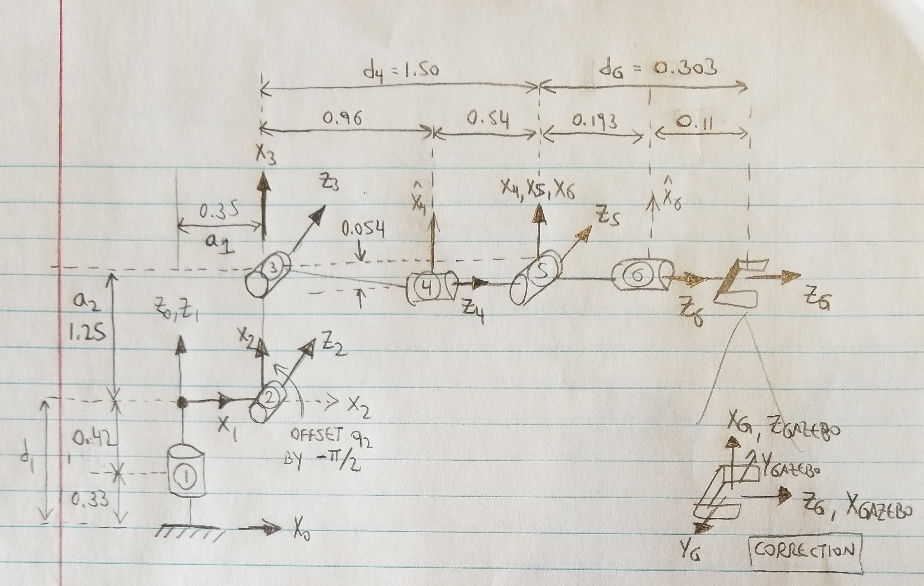
Then, a diagram of the robot was drawn, setting the coordinate frame locations such that the DH parameters are easily determined.
The resulting modified DH parameters were then found by looking at the lengths in the robot URDF file. Note that there is a correction for the angle q2 since its zero configuration corresponds to an angle of pi/2 in the Gazebo simulation.
| Links | alpha(i-1) | a(i-1) | d(i-1) | theta(i) |
|---|---|---|---|---|
| 0->1 | 0 | 0 | 0.75 | q1 |
| 1->2 | -pi/2 | 0.35 | 0 | q2 - pi/2 |
| 2->3 | 0 | 1.25 | 0 | q3 |
| 3->4 | -pi/2 | -0.054 | 1.5 | q4 |
| 4->5 | pi/2 | 0 | 0 | q5 |
| 5->6 | -pi/2 | 0 | 0 | q6 |
| 6->G | 0 | 0 | 0.303 | 0 |
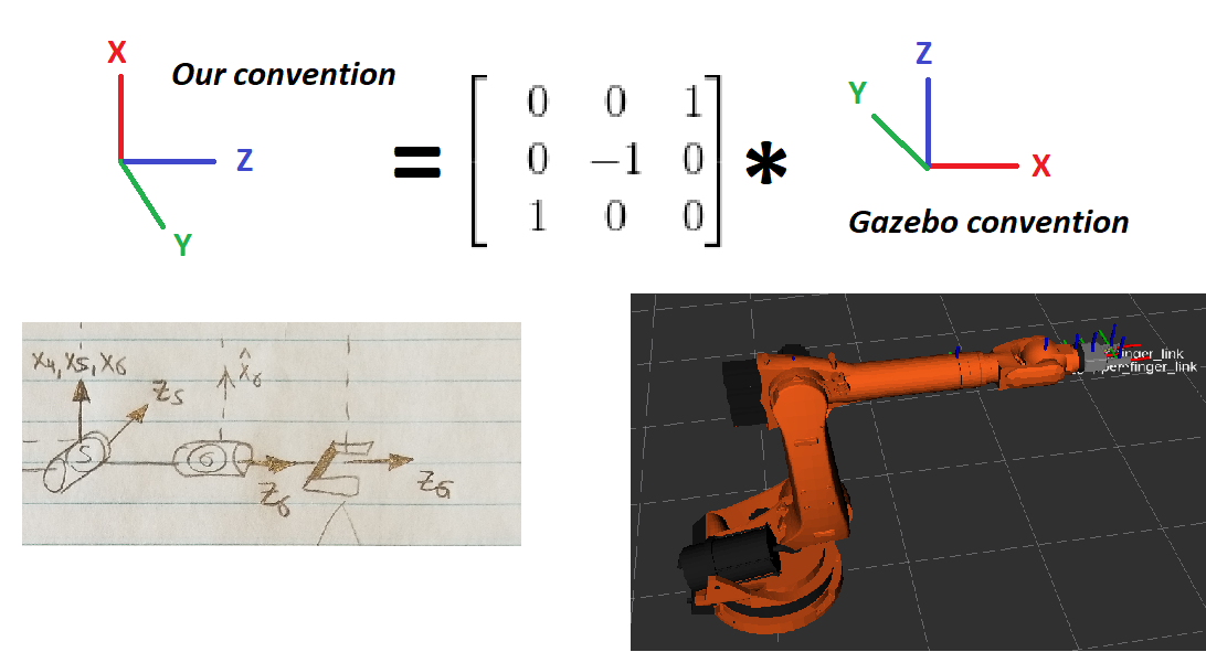
Finally, there needed to be an additional correction matrix since the end effector axis orientation in our schematic is different from that in Gazebo. The URDF file aligned the global world coordinate frame with each joint in zero configuration, whereas we had other rotations that made the DH parameters easier to find.
In contrast to the recommended workflow, we decided to use numpy instead of
sympy to remove the need for symbolic math. Therefore, you will see that
the forward kinematics are defined in separate utility functions called
KR210ForwardMatrix and DHMatrix. These matrices are automatically
calculated given the start and end indices.
An advantage of this code is the flexibility it provides. In the final implementation,
we can directly supply numeric values into the q and params inputs of the following
functions, whereas in the test script we can supply symbolic variables.
# Build transformation matrix from DH parameters
def DHMatrix(alpha,a,d,theta):
    return matrix([[cos(theta), -sin(theta), 0, a],
                   [sin(theta)*cos(alpha), cos(theta)*cos(alpha), -sin(alpha), -sin(alpha)*d],
                   [sin(theta)*sin(alpha), cos(theta)*sin(alpha), cos(alpha), cos(alpha)*d],
                   [0, 0, 0, 1]])


# Build transformation matrix given configuration vector "q" and start and end coordinate frame indices
def KR210ForwardMatrix(q,dhParams,startIdx,endIdx):

    theta = [q[0], q[1]-pi/2, q[2], q[3], q[4], q[5], 0]; # Includes correction to q2 (or q[1])

    # Loop through all the selected indices
    M = eye(4);
    for idx in range(startIdx,endIdx):
        M = M*DHMatrix(alpha[idx],a[idx],d[idx],theta[idx])
    return
In a script called test_kinematics.py, we reused these same functions but also used sympy to generate
the symbolic matrices for the purpose of this report. For example, this is the code to get the first
transformation matrix M1_0:
# Define symbols for all DH parameters
alpha0, alpha1, alpha2, alpha3, alpha4, alpha5, alpha6 = symbols('alpha0:7');
a0, a1, a2, a3, a4, a5, a6 = symbols('a0:7');
d1, d2, d3, d4, d5, d6, d7 = symbols('d1:8');
q1, q2, q3, q4, q5, q6 = symbols('q1:7');

# Package the DH parameters
dhParams = {
       "alpha":[alpha0,alpha1,alpha2,alpha3,alpha4,alpha5,alpha6],
       "a": [a0,a1,a2,a3,a4,a5,a6],
       "d": [d1,d2,d3,d4,d5,d6,d7],
       }
q = [q1,q2,q3,q4,q5,q6];

# Define the a, alpha, and d values to substitute based on the URDF file and derived DH parameters
subsDict = {a0: 0, a1: 0.35, a2: 1.25, a3: -0.054, a4: 0, a5: 0, a6: 0,
        alpha0: 0, alpha1: -pi/2, alpha2: 0, alpha3: -pi/2, alpha4: pi/2, alpha5: -pi/2, alpha6: 0,
        d1: 0.75, d2: 0, d3: 0, d4: 1.5, d5: 0, d6: 0, d7: 0.303};

# Get each individual matrix
M1_0 = KR210ForwardMatrix(q,dhParams,0,1)
print("M1_0")
print(simplify(M1_0))
print(simplify(M1_0.subs(subsDict)))
By following the same for all 7 transformations in the KR210 manipulator, we can get fully symbolic
matrices, as well as matrices with all values substituted except the angles q1 through q6
M1_0
Matrix([
[            cos(q1),            -sin(q1),            0,              a0],
[sin(q1)*cos(alpha0), cos(alpha0)*cos(q1), -sin(alpha0), -d1*sin(alpha0)],
[sin(alpha0)*sin(q1), sin(alpha0)*cos(q1),  cos(alpha0),  d1*cos(alpha0)],
[                  0,                   0,            0,               1]])
Matrix([
[cos(q1), -sin(q1), 0,    0],
[sin(q1),  cos(q1), 0,    0],
[      0,        0, 1, 0.75],
[      0,        0, 0,    1]])

M2_1
Matrix([
[             sin(q2),             cos(q2),            0,              a1],
[-cos(alpha1)*cos(q2), sin(q2)*cos(alpha1), -sin(alpha1), -d2*sin(alpha1)],
[-sin(alpha1)*cos(q2), sin(alpha1)*sin(q2),  cos(alpha1),  d2*cos(alpha1)],
[                   0,                   0,            0,               1]])
Matrix([
[sin(q2),  cos(q2), 0, 0.35],
[      0,        0, 1,    0],
[cos(q2), -sin(q2), 0,    0],
[      0,        0, 0,    1]])

M3_2
Matrix([
[            cos(q3),            -sin(q3),            0,              a2],
[sin(q3)*cos(alpha2), cos(alpha2)*cos(q3), -sin(alpha2), -d3*sin(alpha2)],
[sin(alpha2)*sin(q3), sin(alpha2)*cos(q3),  cos(alpha2),  d3*cos(alpha2)],
[                  0,                   0,            0,               1]])
Matrix([
[cos(q3), -sin(q3), 0, 1.25],
[sin(q3),  cos(q3), 0,    0],
[      0,        0, 1,    0],
[      0,        0, 0,    1]])

M4_3
Matrix([
[            cos(q4),            -sin(q4),            0,              a3],
[sin(q4)*cos(alpha3), cos(alpha3)*cos(q4), -sin(alpha3), -d4*sin(alpha3)],
[sin(alpha3)*sin(q4), sin(alpha3)*cos(q4),  cos(alpha3),  d4*cos(alpha3)],
[                  0,                   0,            0,               1]])
Matrix([
[ cos(q4), -sin(q4), 0, -0.054],
[       0,        0, 1,    1.5],
[-sin(q4), -cos(q4), 0,      0],
[       0,        0, 0,      1]])

M5_4
Matrix([
[            cos(q5),            -sin(q5),            0,              a4],
[sin(q5)*cos(alpha4), cos(alpha4)*cos(q5), -sin(alpha4), -d5*sin(alpha4)],
[sin(alpha4)*sin(q5), sin(alpha4)*cos(q5),  cos(alpha4),  d5*cos(alpha4)],
[                  0,                   0,            0,               1]])
Matrix([
[cos(q5), -sin(q5),  0, 0],
[      0,        0, -1, 0],
[sin(q5),  cos(q5),  0, 0],
[      0,        0,  0, 1]])

M6_5
Matrix([
[            cos(q6),            -sin(q6),            0,              a5],
[sin(q6)*cos(alpha5), cos(alpha5)*cos(q6), -sin(alpha5), -d6*sin(alpha5)],
[sin(alpha5)*sin(q6), sin(alpha5)*cos(q6),  cos(alpha5),  d6*cos(alpha5)],
[                  0,                   0,            0,               1]])
Matrix([
[ cos(q6), -sin(q6), 0, 0],
[       0,        0, 1, 0],
[-sin(q6), -cos(q6), 0, 0],
[       0,        0, 0, 1]])

MG_6
Matrix([
[1,           0,            0,              a6],
[0, cos(alpha6), -sin(alpha6), -d7*sin(alpha6)],
[0, sin(alpha6),  cos(alpha6),  d7*cos(alpha6)],
[0,           0,            0,               1]])
Matrix([
[1, 0, 0,     0],
[0, 1, 0,     0],
[0, 0, 1, 0.303],
[0, 0, 0,     1]])
The full homogeneous transformation matrix from the base to the end effector can be found by multiplying all the matrices above, or by calling the utility function as follows, from index 0 (base) to 7 (end effector).
M = KR210ForwardMatrix(q,dhParams,0,7);
print("Homogeneous matrix from base to end effector")
print(simplify(M.subs(subsDict)))
Which results in...
Matrix([
[((sin(q1)*sin(q4) + sin(q2 + q3)*cos(q1)*cos(q4))*cos(q5) + sin(q5)*cos(q1)*cos(q2 + q3))*cos(q6) - (-sin(q1)*cos(q4) + sin(q4)*sin(q2 + q3)*cos(q1))*sin(q6), -((sin(q1)*sin(q4) + sin(q2 + q3)*cos(q1)*cos(q4))*cos(q5) + sin(q5)*cos(q1)*cos(q2 + q3))*sin(q6) + (sin(q1)*cos(q4) - sin(q4)*sin(q2 + q3)*cos(q1))*cos(q6), -(sin(q1)*sin(q4) + sin(q2 + q3)*cos(q1)*cos(q4))*sin(q5) + cos(q1)*cos(q5)*cos(q2 + q3), -0.303*sin(q1)*sin(q4)*sin(q5) + 1.25*sin(q2)*cos(q1) - 0.303*sin(q5)*sin(q2 + q3)*cos(q1)*cos(q4) - 0.054*sin(q2 + q3)*cos(q1) + 0.303*cos(q1)*cos(q5)*cos(q2 + q3) + 1.5*cos(q1)*cos(q2 + q3) + 0.35*cos(q1)],
[ ((sin(q1)*sin(q2 + q3)*cos(q4) - sin(q4)*cos(q1))*cos(q5) + sin(q1)*sin(q5)*cos(q2 + q3))*cos(q6) - (sin(q1)*sin(q4)*sin(q2 + q3) + cos(q1)*cos(q4))*sin(q6), -((sin(q1)*sin(q2 + q3)*cos(q4) - sin(q4)*cos(q1))*cos(q5) + sin(q1)*sin(q5)*cos(q2 + q3))*sin(q6) - (sin(q1)*sin(q4)*sin(q2 + q3) + cos(q1)*cos(q4))*cos(q6), -(sin(q1)*sin(q2 + q3)*cos(q4) - sin(q4)*cos(q1))*sin(q5) + sin(q1)*cos(q5)*cos(q2 + q3),  1.25*sin(q1)*sin(q2) - 0.303*sin(q1)*sin(q5)*sin(q2 + q3)*cos(q4) - 0.054*sin(q1)*sin(q2 + q3) + 0.303*sin(q1)*cos(q5)*cos(q2 + q3) + 1.5*sin(q1)*cos(q2 + q3) + 0.35*sin(q1) + 0.303*sin(q4)*sin(q5)*cos(q1)],
[                                                                -(sin(q5)*sin(q2 + q3) - cos(q4)*cos(q5)*cos(q2 + q3))*cos(q6) - sin(q4)*sin(q6)*cos(q2 + q3),                                                                  (sin(q5)*sin(q2 + q3) - cos(q4)*cos(q5)*cos(q2 + q3))*sin(q6) - sin(q4)*cos(q6)*cos(q2 + q3),                                     -sin(q5)*cos(q4)*cos(q2 + q3) - sin(q2 + q3)*cos(q5),                                                                                 -0.303*sin(q5)*cos(q4)*cos(q2 + q3) - 0.303*sin(q2 + q3)*cos(q5) - 1.5*sin(q2 + q3) + 1.25*cos(q2) - 0.054*cos(q2 + q3) + 0.75],
[                                                                                                                                                            0,                                                                                                                                                             0,                                                                                        0,                                                                                                                                                                                                              1]])
The resulting matrix for zero configuration, for example, is:
Matrix([
[0,  0, 1, 2.153],
[0, -1, 0,     0],
[1,  0, 0, 1.946],
[0,  0, 0,     1]])
The Inverse Kinematics (IK) problem was solved analytically since the KR210 manipulator has 6 degrees of freedom and a spherical wrist.
Given the requested orientation (roll-pitch-yaw) of the end effector, as well as the length of the wrist, we can back out the location of the wrist center. This wrist center location can be used to calculate the first 3 angles of the manipulator.
# Find the orientation of the end effector in DH coordinates
Rrpy = RotZ(yaw)*RotY(pitch)*RotX(roll)*RotCorr();
nx = Rrpy[0,2];
ny = Rrpy[1,2];
nz = Rrpy[2,2];

# Find the wrist center position
wristLength = dhParams["d"][5]+dhParams["d"][6];
wx = px - wristLength*nx;
wy = py - wristLength*ny;
wz = pz - wristLength*nz;
Using the robot geometry and the location of the wrist center, we can determine the angles theta1 through theta3.
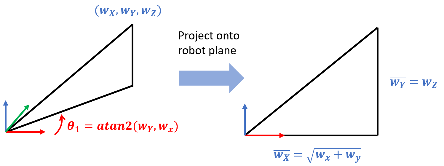
The angle theta1 is the only joint angle that affects the base rotation about the world Z axis, so it can be found by taking the X and Y components of the wrist center.
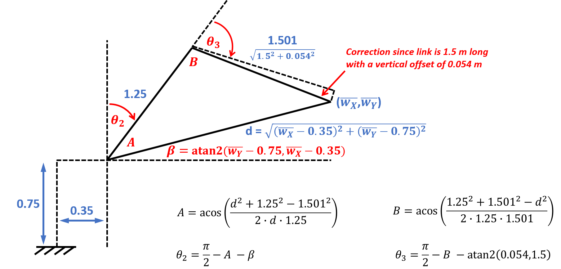
The angles theta2 and theta3 can then be found by taking the manipulator geometry in the robot plane and applying the law of cosines. The schematic below shows the necessary equations, and the corresponding code is below it.
# Geometric IK for joints 1-3
d1 = dhParams["d"][0];
a1 = dhParams["a"][1];
a2 = dhParams["a"][2];
a3 = dhParams["a"][3];
d4 = dhParams["d"][3];
d4_eff = sqrt(d4*d4 + a3*a3);

# Theta1 is defined exclusively by the angle on the X-Y Plane
theta1 = arctan2(wy,wx);

# Theta2 and Theta3 are interdependent and require some trigonometry.
# Refer to the README file for a schematic.
xRef = sqrt(wx*wx + wy*wy) - a1;
yRef = wz - d1;
dRef = sqrt(xRef*xRef + yRef*yRef);
beta = arctan2(yRef,xRef);

angleA = arccos((dRef*dRef + a2*a2 - d4_eff*d4_eff)/(2*a2*dRef))
theta2 = (pi/2) - angleA - beta;

angleB = arccos((a2*a2 + d4_eff*d4_eff - dRef*dRef)/(2*a2*d4_eff))
theta3 = (pi/2) - angleB - arctan2(-a3,d4);
Now that we have the angles theta1 through theta3, we can use forward kinematics to get the homogeneous matrix of the robot at the wrist center. Then, we can invert this matrix to find the transformation matrix from the wrist center to the end effector.
Then, we can take this rotation matrix and find the 3 spherical wrist joint
angles needed to complete the inverse kinematics. This was done using the
euler_from_matrix function, with knowledge that the spherical wrist
(as defined in our convention) is a rotating Z-Y-Z wrist. Also, we also
need to account for the fact that the Y axis in our convention is in the
opposite direction.
# Inverse Orientation for Joints 4-6
q = [theta1, theta2, theta3, 0, 0, 0] # Last 3 values don't matter yet
R0_3 = KR210ForwardMatrix(q,dhParams,0,4)[0:3,0:3] # Do not need 4th dimension
R3_6 = R0_3.T * Rrpy;
theta4, theta5, theta6 = tf.transformations.euler_from_matrix(R3_6,axes='rzyz')
theta5 = -theta5; # Since the rotation is actually z, -y, z
At first, the wrist was rotating wildly because the acceptable values ranged from +pi to -pi. We resolved this issue by ensuring that the theta4 and theta6 angles can only take values between +pi/2 and -pi/2. This way, the wrist joints are prevented from continuously rotating along the planned motion trajectory.
As shown in the code snippet below, flipping the theta4 wrist angle requires theta5 to be flipped in the opposite direction to maintain the same wrist orientation as calculated directly from the matrix.
# Handle multiple theta solutions
# If theta4 is near inverted (pi), flip it by an offset of pi to be near zero
# Note this will require theta5 to be reversed in sign
if (theta4 > 0) and ((pi-theta4) < theta4):
	theta4 = theta4 - pi;
	theta5 = -theta5;
elif (theta4 < 0) and ((theta4+pi) < -theta4):
	theta4 = theta4 + pi;
	theta5 = -theta5;

# Do the same for theta6, which doesn't affect other angles
if (theta6 > 0) and ((pi-theta6) < theta6):
	theta6 = theta6 - pi;
elif (theta6 < 0) and ((theta6+pi) < -theta6):
	theta6 = theta6 + pi;
The inverse kinematics solution adequately solved all test cases within a
few centimeters of error, both in the IK_debug.py script provided, and
when integrated into the final IK_server.py program.
Unfortunately, the Virtual Machine environment prevented looping
through all test cases continuously in RViz, as respawning a new object
after the first pick-and-place task was complete somehow generated an
error message about the trajectory_sampler process dying.


