Colorway can be installed from Github using the devtools package:
devtools::install_github("hypercompetent/colorway")
color_lgl() and color_which() provide an easy way to test color values in RGB/HSV space:
color_vec <- c("#FF0000","dodgerblue","orange","808080","#000000")

# Which colors have an R value > 0.5 in RGB space (scaled between 0 and 1)?
color_which(color_vec,
            r > 0.5)
[1] 1 3 4

# Which colors have R or G > 0.3 in RGB space?
color_which(color_vec,
             r > 0.3 | g > 0.3)
[1] 1 2 3 4

# Which colors are dark (low V in HSV space)?
color_lgl(color_vec,
          v < 0.2)
[1] FALSE FALSE FALSE FALSE  TRUE

# Which colors are bright, saturated red?
color_lgl(color_vec,
          r > 0.7 & s > 0.7 & v > 0.7)
[1]  TRUE FALSE  TRUE FALSE FALSE
Colorway provides functions for building and inspecting color palettes.
build_palette() will generate a palette of similar colors based around a seed color, and provides additional outputs for evaluating the selected palette:
blue_palette <- build_palette("dodgerblue")
The output of build_palette() is a list with 5 entries.
palette is a set of 10 colors related to the seed color:
blue_palette$palette

[1] "#1B6CE6" "#1EC6FF" "#175DBF" "#1E90FF" "#1E4DFF" "#177BBF" "#1545B3" "#1B90E6" "#1587B3"
pallette_plot is a plot showing these selected colors.
blue_palette$palette_plot
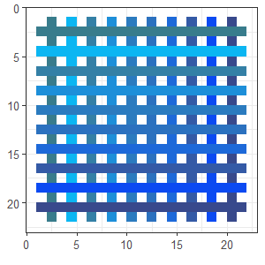
weave is a plot showing the overlap between all colors in the palette, which is useful for determining if colors in the set are distinct enough.
blue_palette$weave
Additional related colors are provided in colorset, which is a pool of 100 colors from which the 10 palette colors are selected:
blue_palette$colorset

  [1] "#11748C" "#127D99" "#1487A6" "#1590B3" "#179ABF" "#18A3CC" "#1AACD9"
  [8] "#1BB5E6" "#1DBDF2" "#1EC6FF" "#116C8C" "#127599" "#147EA6" "#1587B3"
 [15] "#178FBF" "#1898CC" "#1AA0D9" "#1BA8E6" "#1DB1F2" "#1EB9FF" "#11658C"
 [22] "#126D99" "#1475A6" "#157DB3" "#1785BF" "#188DCC" "#1A95D9" "#1B9CE6"
 [29] "#1DA4F2" "#1EABFF" "#115D8C" "#126599" "#146DA6" "#1574B3" "#177BBF"
 [36] "#1882CC" "#1A89D9" "#1B90E6" "#1D97F2" "#1E9EFF" "#11568C" "#125D99"
 [43] "#1464A6" "#156AB3" "#1771BF" "#1878CC" "#1A7ED9" "#1B84E6" "#1D8AF2"
 [50] "#1E90FF" "#114E8C" "#125599" "#145BA6" "#1561B3" "#1767BF" "#186DCC"
 [57] "#1A72D9" "#1B78E6" "#1D7DF2" "#1E83FF" "#11478C" "#124D99" "#1452A6"
 [64] "#1558B3" "#175DBF" "#1862CC" "#1A67D9" "#1B6CE6" "#1D70F2" "#1E75FF"
 [71] "#11408C" "#124599" "#1449A6" "#154EB3" "#1753BF" "#1857CC" "#1A5BD9"
 [78] "#1B60E6" "#1D64F2" "#1E68FF" "#11388C" "#123C99" "#1441A6" "#1545B3"
 [85] "#1749BF" "#184CCC" "#1A50D9" "#1B53E6" "#1D57F2" "#1E5AFF" "#11318C"
 [92] "#123499" "#1438A6" "#153BB3" "#173EBF" "#1842CC" "#1A44D9" "#1B47E6"
 [99] "#1D4AF2" "#1E4DFF"
The colorset is plotted in colorset_plot:
blue_palette$colorset_plot
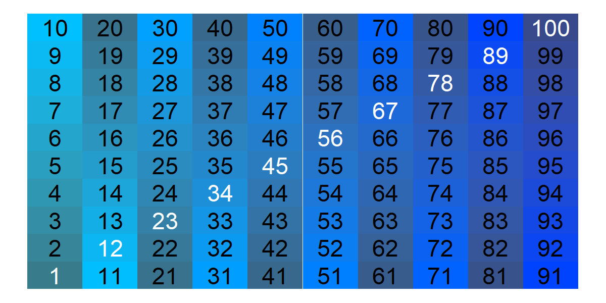 White numbers indicate which colors were selected for the
 palette.
The varibow() function generates a set of colors similar to base R's rainbow() function, but with more variation in saturation and value.
I used varibow() to generate colors for Rosenberg and Roco, et al (2018), published in Science:
 Note that the colors look a bit different here due to conversion to CMYK colorspace.
Here's a simpler example of function usage:
varied_colors <- varibow(10)
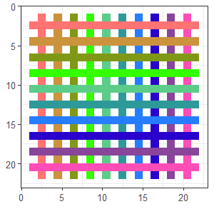
These (or any set of colors) can be viewed with weave_plot():
weave_plot(varied_colors)
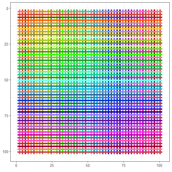
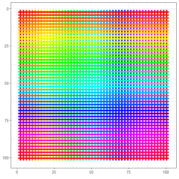
varibow() is especially useful when you need a large set of diverse colors in which adjacent colors are easy to distinguish. Let's compare rainbow() and varibow() for 50 colors:
varibow_50 <- varibow(50)
rainbow_50 <- rainbow(50)

varibow_weave <- weave_plot(varibow)
rainbow_weave <- weave_plot(rainbow)

varibow_weave
rainbow_weave
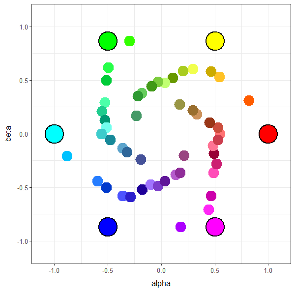
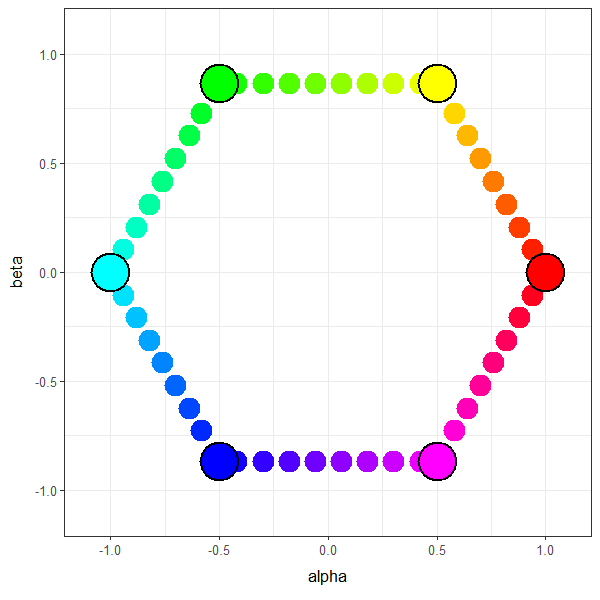
Another view on color palettes is provided by colorspace_plot(). Colorspace plot converts colors to a 2-dimensional Hue and Chroma representation, as described here: https://en.wikipedia.org/wiki/HSL_and_HSV#Hue_and_chroma. This gives a good view of the overall color coverage of a set of colors:
colorspace_plot(varibow_50)
colorspace_plot(rainbow_50)
values_to_colors() provides a convenient method for translating numeric values to a color ramp. This is convenient for custom heatmaps.
values <- c(1,4,10,17,20,35,60)
colors <- values_to_colors(values)

ggplot() +
  geom_tile(aes(x = 1:8, y = 1,
                fill = colors)) +
  scale_fill_identity()
You can easily change the colorset:
colors <- values_to_colors(values,
                           colorset = c("magenta","black","yellow"))

ggplot() +
  geom_tile(aes(x = 1:8, y = 1,
                fill = colors)) +
  scale_fill_identity()
By default, the minimum and maxium values used for the ends of the color mapping are automatically determined by the input values. One can also manually set minimum and maximum values to ensure equal scaling across multiple sets of values:
colors <- values_to_colors(values,
                           colorset = c("magenta","black","yellow"),
                           min_val = 10,
                           max_val = 80)

ggplot() +
  geom_tile(aes(x = 1:8, y = 1,
                fill = colors)) +
  scale_fill_identity()

