This repository contains the source code for training a deep neural network to perform human pose estimation from scratch. A brief excerpt from our final report is copied below.
Our model is deployed online here! Unfortunately due to Streamlit's deployment website's minimum Python version no longer compatible with Tensorflow 1.15.x, the website is turned off until it can be fixed. Please be aware that the model only supports single-person human pose estimation. In the event there are multiple people in the frame, the model will label the skeleton of the center-most person.
Our final report is linked here.
Feel free to check out our demo photos, or upload your own to try out. If you encounter any issues, please open an issue in this repository.
If you upload your own photos, please crop them so the person of interest is relatively centered, taking up approxiately 70-90% of the vertical space. The model is robust to cropped image boundaries being black, so don't worry about cropping to an irregular shape. We'll automatically center the image in our pre-processing pipeline.
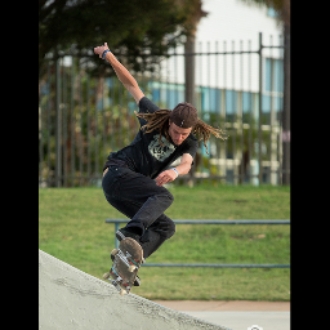
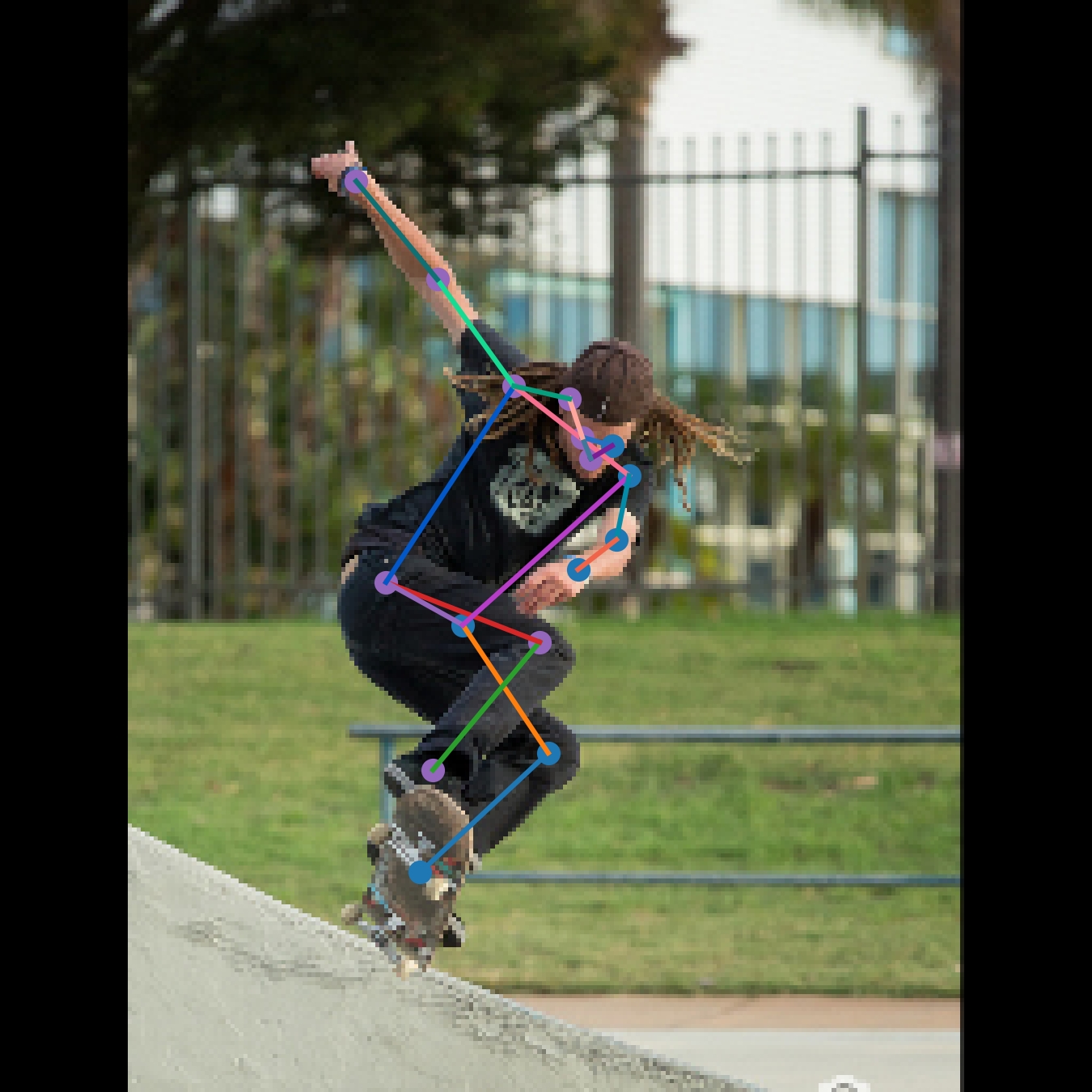
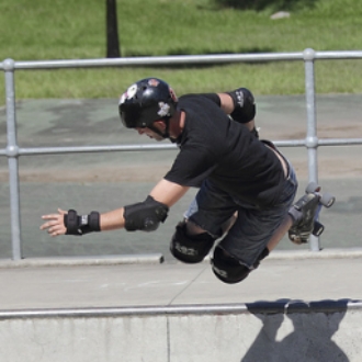
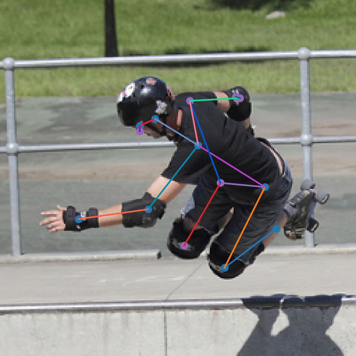
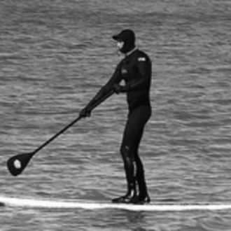
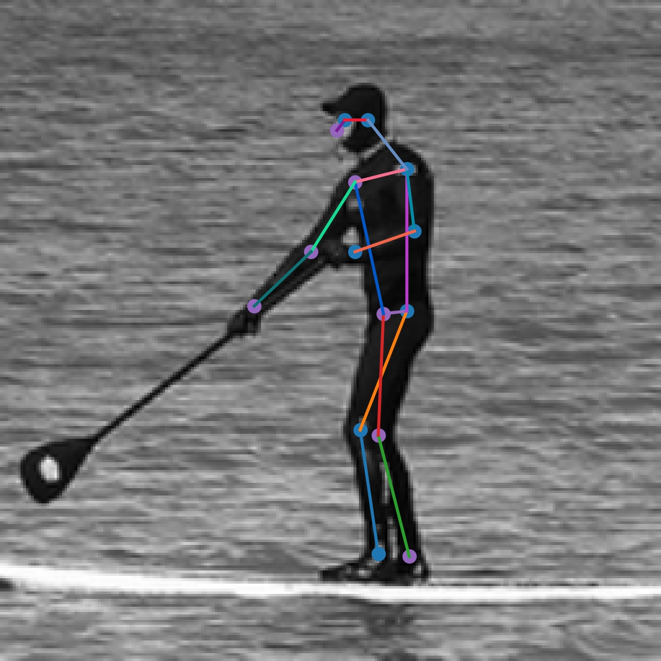
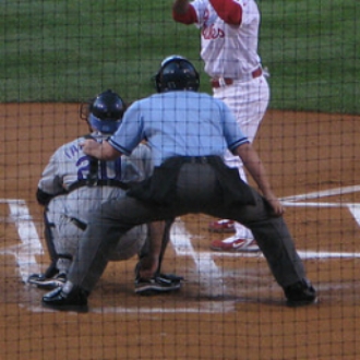
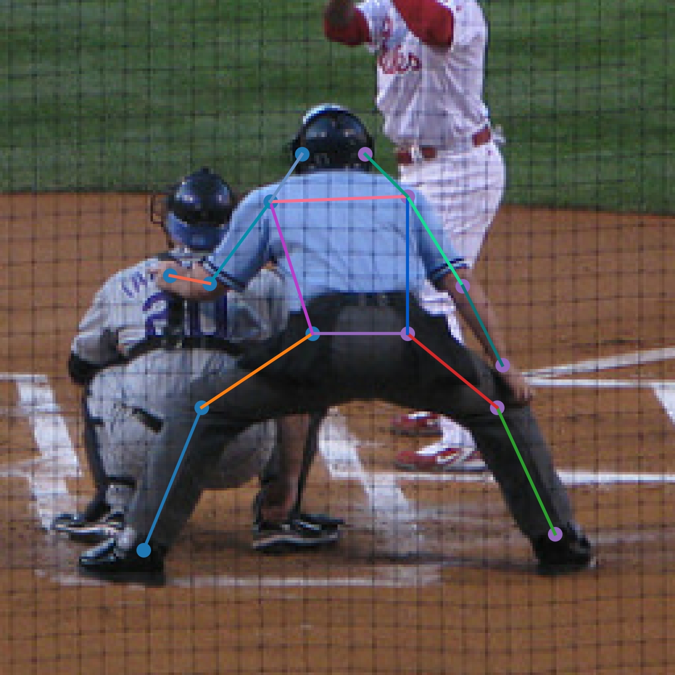
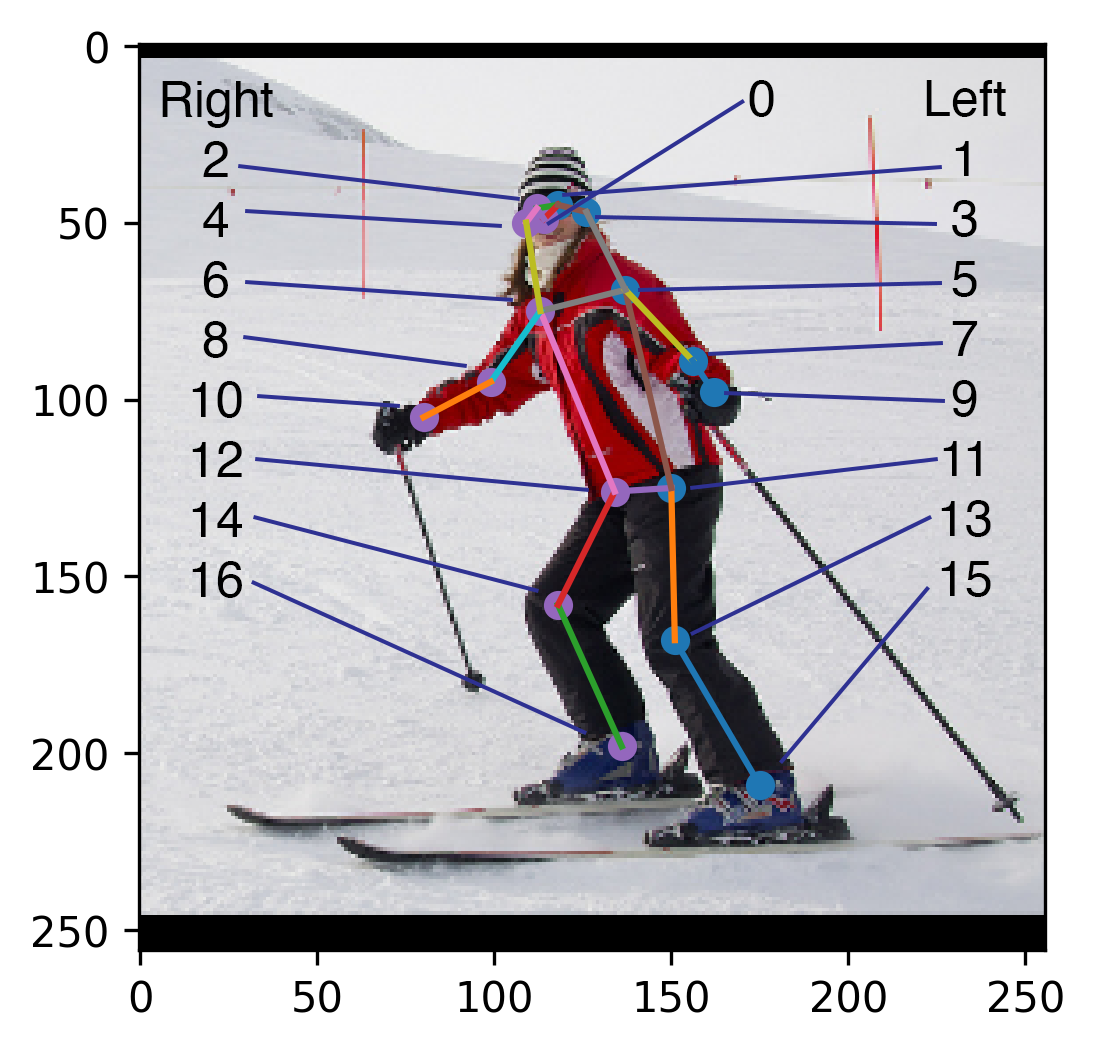
The following outputs show the predictions from a 4 hourglass stack model, epoch 107. The input image is on the left. The prediction image is on the right. The right-side body keypoints are magenta, and the left-side body keypoints are blue. Each joint-joint connection has its own assigned colour that is consistent across images. Keypoints that are not seen by the model are not displayed. These sample images are from the COCO 2017 dataset.
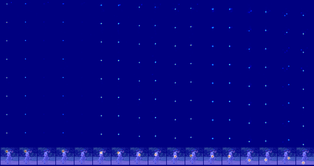
The model's unprocessed output is a series of heatmaps, one for each joint. Since intermediate supervision was used, we also visualize the heatmaps in the inner layers. To read the heatmap, each column represents one of the 17 joints. Each row represents a layer. The first layer is the first row, and the last layer is the second-last row. The final prediction for a particular joint is overlayed on the input image and displayed on the last row.
Notice that the model refines its predictions as we proceed deeper into the layers. For example, the first row predictions often identify both ankles, wrists, or other joints that are difficult to immediately discern left and right. Each image below that shows the model deciding which joint corresponds to the person's left/right.
The columns, if numbered in increasing order from left to right (0, 1, 2, ..., 16), correspond to the joints in this labelled figure.
4-layer hourglass, epoch 107
8-layer hourglass, epoch 70
To better see the model performing refinements, we retrieve a heatmap output from the early stages of training, epoch 15 of 107. Notice the ankles and knees (rightmost 4 columns). In the first layer, both are identified. As we proceed deeper into the model, it uses context and other cues to determine which side is the person's left and right.
- init submodules
git submodule update --init --recursive- install requirements
pip3 install -r requirements.txt- install dataset (requires just under 30 GB after unzipping, but will require at least 45 GB free disk space to unzip a ~18 GB training set)
bash ./scripts/coco_dl.sh- If you encounter any pip issues installing
pycocotools, manually install directly a version that's been updated for Python 3. See this Stack Overflow pycocotools question
pip3 install git+https://github.com/philferriere/cocoapi.git#subdirectory=PythonAPI- If you encounter issues running the evaluation code (specifically for OKS), you may need an earlier version of
numpy:
pip3 install numpy==1.17.0Human pose estimation (HPE) is the task of identifying body keypoints on an input image to construct a body model. The motivation for this topic was driven by the exciting applications of HPE: pedestrian behaviour detection, sign language translation, animation and film, security systems, sports science, and many others. HPE shares many challenges with typical computer vision problems, such as intra-class variations, lighting, perspective, and object occlusions. It also faces challenges unique to HPE such as strong articulations, small and barely visible joints, and self-occlusions from overlapping joints. This report discusses a stacked hourglass network architecture that was developed and trained from scratch to achieve performance comparable with models on the COCO leaderboard from late 2016. This work uses the existing COCO 2017 Keypoint Detection dataset. The final model performs very well on most images, especially those containing well-separated people with the subject centered in frame. It struggles with images containing highly overlapped people or heavily occluded or articulated keypoints.
Our group created a stacked hourglass network that was trained on the Common Objects in Context (COCO) dataset. Our network predicts a maximum of 17 keypoints spanning the full human body on a 2D image. A number of challenges make HPE a difficult problem domain; these challenges include variability in human appearance and physique, environment lighting and weather, occlusions from other objects, self-occlusions from overlapping joints, complexity of movements of the human skeleton, and the inherent loss of information with a 2D image input. This largely unsolved problem enabled us to explore many novel and creative approaches, enriching our learning experience. We are excited to report the results we yielded.
The following sections were summarized from the final report. This report is not fully complete, and will be available later. Please feel free to reach out to view it sooner.
HPE systems can be categorized into 2D vs 3D and single-person vs multi-person. To improve the feasibility of our project, we have focused on single-frame single-person monocular RGB images. Current state-of-the-art techniques for 2D single-person HPE can be categorized into two categories: regression on absolute joint position, or detection on joint locations with heat maps. Since a direct mapping from the input space to joint coordinates is a highly non-linear problem, heat-map-based approaches have proven to be more robust by including small-region information. Thus, we have chosen the heat map approach.
There are three different types of models used with full body HPE: kinematic, contour, and volumetric, as shown in Fig. \ref{fig:body_model} \cite{Chen_2020}. A kinematic model resembles a stick-figure skeleton. The contour model consists of 2D squares and rectangles that represent the body, and the volumetric model represents the body with 3D cylinders. The kinematic model is the simplest model to perform loss metric computations, and thus is preferred by our group as a scope-limiting decision to simplify the problem space. Our goal is to predict a kinematic model for the individual in each picture.
We chose to use the COCO Keypoint dataset \cite{coco_data}. This dataset consists of 330 K images, of which 200 K are labelled. There are pre-sorted subsets of this dataset specific for HPE competitions: COCO16 and COCO17. These contain 147 K images labelled with bounding boxes, joint locations, and human body segmentation masks. We originally considered using DensePose, which is a highly detailed manually annotated subset of the COCO dataset, but found it does not offer joint coordinate labels. Another popular dataset is the MPII dataset, which consists of 41 K labelled images split into 29 K train and 12 K test. We originally planned to use this for validating our model’s performance.
There are 66,808 images in the COCO dataset containing a total of 273,469 annotations. As shown in Fig. \ref{fig:coco_metrics} a), most of the annotations in the COCO dataset do not have all 17 keypoints of the body labelled. The model should not expect a perfect human image with all keypoints visible in frame. The model should instead output a dynamic number of keypoints based on what it can find. But what is the purpose of an annotation with 0 to 4 labelled keypoints? Fig. \ref{fig:zero_kp_images} shows examples of these annotations with few labelled keypoints. Clearly the bounding boxes of these annotations denote people, but because there are not many keypoints, these examples may confuse the model. If the model should be shown examples with 0 keypoints, then images that do not contain people would be more helpful. 5 keypoints was chosen intuitively as the minimum number of keypoints for a usable example; any less and the image rarely contains enough information to clearly make out a person. Therefore, despite the fact that 0-4 keypoint annotations make up 48.86% of the total COCO dataset annotations, these annotations were filtered out during training.
Even though our goal is a model that estimates the pose of a single person in the image, 61.28% of the COCO images contain more than one annotated person. The annotations per image are broken down in Fig. \ref{fig:coco_metrics} b). It would be desirable if multi person images did not need to be discarded, so cropping to a bounding box converts a multi person image into a single person image. Keeping these images with multiple people has many benefits. The main benefit is training the model to label the person in the direct center of the image, in cases where multiple people (and thus multiple joints) are present. This is a more realistic use of the model, as it is unlikely that real-world images are always single-person. The other benefit is training on a much larger dataset.
The pre-processing responsibilities of the data generator include: cropping to the ground truth bounding box of a person, resizing to the models input resolution and dimensions, performing random data augmentation, and converting ground truth annotations for each keypoint to a Gaussian heatmap for the cropped images. Fig. \ref{fig:data_gen_ex} shows an example of the transformations. Fig. \ref{fig:data_gen_ex} only shows the cropping for one person but since there are 4 annotated people, the image would get split into 4 images, each centered on the person of interest. Fig. \ref{fig:data_gen_ex} also only shows the heat map of the left hand, but since COCO annotations contain 17 keypoints, it produces 17 heatmaps per annotation.
The network is based on Newell 2016's stacked hourglass network. It consists of a series of stacked U-Nets. The network gets its name because the U-Nets resemble hourglass structures. Each U-Net, shown in Fig. \ref{fig:single_hourglass} is a lightweight encoder-decoder structure that consists of residual blocks with either convolution or upsampling applied for the encoder and decoder stages, respectively. Unlike typical U-Nets that have proven successful for problem domains such as semantic segmentation, this network does not use unpooling or deconvolutional layers during the decoder stage. Instead, nearest neighbour upsampling is used. Skip connections link feature levels of the same spatial resolution in the encoder and decoder stages. This structure allows the network to combine information from deep abstract features, and local high-resolution information.
The input to the entire model is a RGB image of resolution 256x256. Since performing operations at original resolution is expensive in compute and memory, all the internal hourglass stacks have a max resolution of 64x64. Thus, between the input layer and the first hourglass block, the input resolution is brought down from 256x256 to 64x64 by using the following operations: a 7x7 convolutional layer with stride 2, a residual module, and max pooling.
The input to each hourglass block is at a resolution of 64x64. The encoder block performs top-down processing, where the image spatial domain is decreased while increasing feature depth. After each convolution block, max pooling is applied to reduce in spatial size. The network also branches off at the pre-pooled resolution to apply more convolutions to form the \textit{skip connections}. At the smallest stage in the middle of the hourglass, which is denoted the \textit{bottleneck}, the network is at a resolution of 4x4 pixels. Here, the convolution operations can compare global features in the image. To reconstruct the original resolution, the network applies nearest-neighbour upsampling and joins feature information from the skip connections. The final resolution is identical to the input at 64x64, and the network is fully symmetric.
At the output resolution, the network predictions are constructed by applying two rounds of 1x1 convolutions to the extracted features. This forms a series of 17 one-channel heatmaps, one for each joint, where the intensity of the pixel value corresponds to the probability that a joint is found at that location. This intermediate prediction is added with the feature map and used as input to the next layer. In essence, each block in this architecture performs a refinement of predictions generated by the previous block. The number of hourglass blocks does not affect the output resolution, since each block is symmetric.
Deep networks can often suffer from vanishing gradients, which is where the gradients of the loss function approach zero deep into the network. This is often due to the activation functions, such as sigmoid, having a range of values where the gradient is extremely small. Since these gradients multiplied together using the chain rule during backpropagation, this can cause the gradient to disappear deep into the networks. These gradients are used to update the weights during backpropagation, so vanishing gradients can stall learning and result in a poorly performing network.
To mitigate this problem, the network architecture uses both residual blocks and intermediate supervision. Residual blocks adds both the modified output from the convolution and activation operations, and the original values. This permits an alternative path for gradients to flow through the network. Since this network is highly symmetric, intermediate supervision was used as well. The ideal output for a perfect network would have each hourglass block output identical heatmaps, we extract intermediate prediction heatmaps to perform loss function evaluations. This allows the network to re-introduce gradients deep into the network, reducing the risk of vanishing gradients.
To gain insight into our model's predictions, we first visualized and compared the 17 output heatmaps, corresponding to COCO joints, from each successive hourglass layer with the image's ground truth heatmaps. This is shown for a 4 layer hourglass model in Fig. \ref{fig:Visualization} a). This figure shows the architecture refinement in the top right corner, where the model originally predicts two points on the heatmap with approximately equal brightness until gaining more confidence on one point in the final hourglass layer. Often, this refinement would help distinguish the models confusion between the left and right of each joint. In order to evaluate the model, we converted the predicted heatmaps back into COCO formatted keypoints. This conversion was accomplished by first upscaling each heatmap from 64x64 to the original image size of 256x256, then using a gaussian filter to blur each heatmap, and finally choosing the maximum point in the heatmap with non-maximum suppression by forcing values less than the determined threshold of 0.04 to 0. One set of keypoint coordinates is determined for each heatmap and later used for evaluating the model. For qualitative assessment of the model, a method to visualize the estimated keypoints in a skeleton overlayed on the input image was implemented, shown in Fig. \ref{fig:Visualization} b).
The goal of this project was to develop an HPE model that can perform with high accuracy and generalize well to unseen data. The success of the model was measured using 2 quantifiable metrics common to the HPE literature \cite{Babu_2019}.
The first metric that was implemented for evaluation was OKS. We computed this metric across epochs to determine our models with the highest accuracy. Each model has rapid improvement in the first 5 epochs and further epochs have slower and more gradual improvement as seen in Fig. \ref{fig:OKS_graph_hg4_flip}. Our highest performing model was able to achieve an OKS primary challenge metric score of 0.575 and an OKS loose metric score of 0.795. This score is competitive with models on the COCO leaderboard from 2016. Using horizontally flipped images and taking the average bumped the scores by 3-5% for this metric. OKS is commonly reported in the literature in terms of AR (average recall) and AP (average precision). It was implemented using the COCO Python API \cite{coco_keypoints}. The API allows for evaluation of results and the ability to compute precision and recall of OKS across scales. It required that our model outputs be formatted according to the COCO keypoint detection standard \cite{coco_format_results}. Beyond model evaluation, the API also provided methods for detailed analysis of errors with plots that were explored and aided in parameter tuning.
The second metric was PCK \cite{Cbsudux_2019} which we implemented ourselves, separately from the COCO evaluation API. There are a number of variations of PCK, and from our research it does not appear to be a standardized metric. PCK considers a detected joint as correct if the distance between the predicted and the true joint is within a specified threshold. We implemented a variation of PCK@0.2, which uses a threshold of 20% of the torso diameter from the ground truth keypoints. Since the literature is not clear on the metric's behaviour when one or both hip points are not present, we implemented a secondary measure of 20% of the head diameter. Our default case is an empirically determined average hip width from the dataset if neither a torso or head was detected in the image. Our highest performing model achieved 0.787 on average for each joint PCK. The model PCK over epochs is graphed in Fig. \ref{fig:PCK_graph_hg4_no_flip}. The results broken down for each joint are specified in Table \ref{table:pck_breakdown}.
