Tackling Lane Following with Vehicles using Semantic Segmentation {#demo-semantic-segmentation status=beta}
This is the description of the "Lane Following with Vehicles (LFV) using Semantic Segmentation" demo.
Contributor(s): Rey Reza Wiyatno and Dong Wang
Requires: Fully set up Duckiebot or have done the instructions in the Duckiebot Operation Manual and Lane Following Demo.
Requires: have done the Getting Started instructions in The AI Driving Olympics page.
Results: A Duckiebot capable of performing lane following with other vehicles using semantic segmentation at its core. The Duckiebot should stop moving if the other vehicles are too close to the Duckiebot.
The goal of the LFV challenge is to perform lane following without hitting other possibly moving vehicles within the same environment. This means, the Duckiebot needs to know where the lanes and obstacles are located, decide what to do next, and execute the action. The core of this approach it to leverage the generalizability of learning-based semantic segmention model to find where the lines (or roads) and obstacles are (e.g., Duckiebots, duckies, cones, etc.) in the image space. We can then ground project these information so we know the location of the lines and obstacles in the robot's coordinate frame. Once we have the ground projected points, we can compute where to go next (i.e., compute follow point) and use this follow point as the input to our controller (which in our case is the pure pursuit controller) that will predict the linear and angular velocity for the robot to execute. In the following subsections, we will discuss each of these components in more detail.
We use deep learning based model to perform semantic segmentation since they are currently considered to be one of the best methods to perform this task. Using learning-based semantic segmentation model has advantages when compared to classic approaches such as color-based methods when detecting Duckiebots and duckies (e.g., assuming red for Duckiebots and yellow for duckies). For example, color-based methods are not able to differentiate between Duckiebots and red lines, or duckies and yellow lines. One may argue that deep learning based semantic segmentation models are typically large and may not run in real time if we do not have access to a GPU. Indeed, we initially used a larger capacity segmentation model called The One Hundred Layers Tiramisu and faced difficulties when making submissions to the AI-DO. We fixed this problem by implementing the model based on the MobileNets and the FCN that uses combinations of depthwise and pointwise convolutions for faster computation. After these changes, we can make submissions to the AI-DO without problems and our whole pipeline can run entirely on CPU.
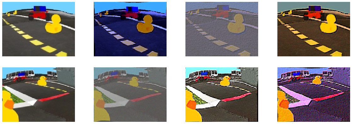
In addition, we also did not want to manually label thousands of training images with their segmentation maps. Instead, we would like to train our model on images that we can gather from the Duckietown simulation since we can generate the segmentation maps for free. The main challenge with this is that our segmentation model may easily overfit to the simulated image domain, and it may not work well to segment real world images. In other words, we would need to perform simulation-to-real transfer (or in short, sim-to-real). We did this by performing one of the most popular sim-to-real methods: domain randomization. Domain randomization works by training our model on images that have been randomly transformed, while still using the same labels from the original image. The hope is for the model to eventually be able to generalize well across domains. Note that we should still make sure the image to maintain its semantic meaning after being transformed. We refer readers to Tobin et al. (2017) for the primer about domain randomization.
Although the Duckietown simulation allows us to do domain randomization, we added more transformations into our domain randomization pipeline to make the images more diverse. These additional transformations include randomization of hue level, saturation level, elastic transformation, contrast, gaussian noise, sharpening, and embossing. We use the imgaug library to apply these additional transformations. Moreover, inspired by the application of robust optimization in adversarial machine learning, where training machine learning model exclusively on adversarial examples rather than the inputs that we may see during test time (i.e., inputs from the training set) has been shown to increase generalizability Madry et al. (2017), we only trained our segmentation model exclusively on the transformed images.
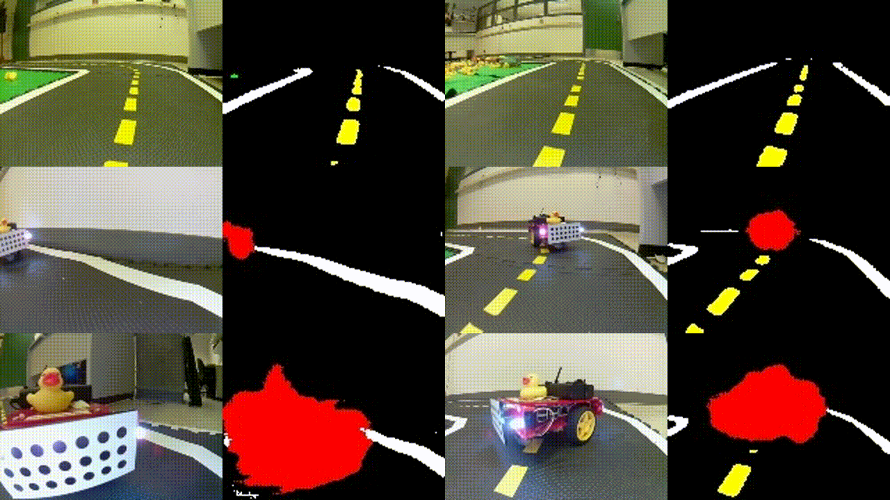
Samples of images before (most left images) and after domain randomization.Finally, we finetuned the trained segmentation model using 230 labeled real world images. From the results we saw above, we can see how the segmentation model can indeed perform well on real world images after being finetuned. The trained models can be found in nodes directory. We also include a notebook that explains how to train the segmentation model.
This functionality is implemented as a ROS node that subscribes to the camera image topic and publishes the segmentation map as another image topic.
EXPERIMENTAL:
In addition to domain randomization, we also experimented with different sim-to-real approaches. These include variants of adversarial domain adaptation and Randomized-to-Canonical Adaptation Networks or RCANs. Our early attempts did not work too well, so we decided not to spend too much time on it due to time constraints. Nevertheless, both of these methods are interesting to try and may produce better results compared to domain randomization if trained properly, although one may need to take into account the extra computation needed to run another neural network model.
This video demonstrates our early attemps using RCANs. From left to right: camera image, predicted canonical image, and predicted segmentation map. We can see it does not perform too well.The goal of the ground projection module is to get the location of points that belong to some classes (e.g., lines, Duckiebots, etc.) in the robot's coordinate frame. Thus, the ground projection module takes the segmentation map that is published by the lane and obstacle detection module as the input. In our implementation, rather than ground projecting all the points, we apply multiple filters so we can only ground project the useful ones.
First, we disregard anything above the horizon and only consider the bottom 2/3 of the segmentation map. We also disregard all points that belong to "background and others" (BLACK points) and "red line" (PURPLE points) classes since they are not useful in LFV challenge. Moreover, in order to compensate for possibly noisy segmentation model, we ignore a class if the number of points that belong to this class is below than a certain threshold.
Next, we filter the points further based on some heuristics that we know from the task we are doing (i.e., lane following while not hitting obstacles). We disregard points that belong to "white lines" if they are located to the right of the yellow lines since we only want our robot to be within the right lane. For "obstacles" points (i.e., GREEN and RED points), we only consider those that are located between yellow and white lines (i.e., we do not need to worry about obstacles that are not within the lane).
To further reduce the noise in white and yellow lines, we apply RANSAC to fit a straight line for both the WHITE and YELLOW points. A better option is to fit a higher order polynomials (e.g., cubic) line. We attempted to do this, but did not get a good results in time. However, we encourage curious readers to implement this in order to improve the overall performance.
Finally, we ground project all the remaining WHITE and YELLOW points onto the ground since we know that white and yellow lines are indeed part of the ground plane. For GREEN and RED points, we only ground project the points that correspond to the bottom of the obstacles. The implementation of the ground projection mostly follows the one available in the ground_projection package. The ground projected points will then be used to compute the follow point (next subsection).
To compute where to go next, given all the ground projected points, we consider cases when we see obstacles or not.
For the case when we do not see obstacles, there are cases when we see both white and yellow lines, only yellow line, and only white line. For the case when we see both lines, we compute the centroid from each of the lines, and compute the follow point as the middle point between these two centroids. If we only see one of these lines, then we compute the follow point as the centroid of the line added with some offset value so that the follow point is located in the middle of the lane.
For the case when we see obstacles, we may consider all combinations of classes that may appear (e.g., WHITE-YELLOW-RED, WHITE-YELLOW-GREEN, WHITE-YELLOW-GREEN-RED, etc.). For the LFV challenge, we can consider only the cases when other Duckiebot appears (i.e., there exist RED points). That is, we check the distance of the closest RED point to our Duckiebot. If the distance is lower than certain threshold value, we consider the other Duckiebot to be too close to our robot and the follow point should be set at (0,0) (i.e., the origin of our robot's coordinate frame) to make our Duckiebot stops moving. With this approach, if there is a moving Duckiebot in front of our Duckiebot, our robot will always maintain its distance from the other vehicle while keep following the lane.
EXPERIMENTAL:
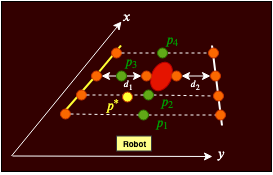
Beyond the LFV challenge, although we have not fully tested this yet, we also thought of a method that will allow our Duckiebot to avoid and pass a static obstacle if there is enough space around the obstacle. For example, this can be useful if there is a duckie located near white or the yellow lines.
Illustration of the proposed follow point (p*) calculation. First, we sample multiple points along the x-axis on both white and yellow lines (the orange points). When there is no obstacle, we calculate the candidate follow points (e.g., p1, p2, p4) by taking the mean from each pair of the sampled orange points. When there is an obstacle, we would like to see whether the opening on one side of the obstacles is larger than the other side. In this particular case, since d1 is larger than d2, we determine p3 by calculating the mean between the point on the yellow line and the point on the left side of the obstacle. Finally, we ignore p4 since it is located further than where the obstacle is, and calculate the follow point as the center of p1, p2, and p3.Pure pursuit controller is a geometric path following controller whose goals are to align the heading of the vehicle with the path heading and to eliminate crosstrack errors from the reference path. In standard pure pursuit controller, we usually set the velocity of the vehicle to be constant, so that we can compute the required angular velocity that will take the vehicle from its current position to the follow point (or sometimes referred to as the look ahead point). For example, in our case, given a follow point, we can calculate the angle required for our robot to face the follow point, which can then be used to calculate the required angular velocity (i.e., the angular velocity is calculated as a function of this angle, velocity, and the look ahead distance). We then added some additional features on top of the standard pure pursuit controller. These include a function to modify the velocity as a function of angle required for our robot to face the follow point. This was done so our robot decelerate when it needs to make a sharp turn, and accelerates during straight lane. A parameter to change the profile of this relationship was also added (e.g., quadratic, cubic, etc.). To have more control, the gains and offsets when detecting yellow or white lines only were set to be different. These parameters can then be adjusted based on trial and error.
The easiest way to run this demo is to clone our fork of AIDO LF baseline Github repository. However, we also made our package available for those interested (see below in Extras).
Clone our fork of AIDO LF baseline Github repository
laptop $ git clone -b daffy git@github.com:rrwiyatn/challenge-aido_LF-baseline-duckietown.git --recursive
Update submodules
laptop $ cd challenge-aido_LF-baseline-duckietown
laptop $ git submodule init
laptop $ git submodule update
laptop $ git submodule foreach "(git checkout daffy; git pull)"
Go to 1_develop directory
laptop $ cd challenge-aido_LF-baseline-duckietown/1_develop
We have provided a map file with two moving Duckiebots in challenge-aido_LF-baseline-duckietown/assets/. To make this the default map, copy this file into challenge-aido_LF-baseline-duckietown/1_develop/simulation/src/gym_duckietown/maps/. Assuming we are currently in challenge-aido_LF-baseline-duckietown/1_develop, we can run:
laptop $ cp ../assets/loop_obstacles.yaml simulation/src/gym_duckietown/maps/
Then, we need to build and run Docker
laptop $ docker-compose build
laptop $ docker-compose up
Next, see the output of our terminal after running docker-compose up, find the line that says http://127.0.0.1:8888/?token={SOME_LONG_TOKEN} and open it in your browser, this should bring us to a Jupyter notebook homepage. Click on a dropdown that says "New" on the top-right corner, and click on "Terminal". This will open a terminal in a new tab. Go to the terminal that we just created, and run the following
laptop-container $ source /opt/ros/melodic/setup.bash
laptop-container $ catkin build --workspace catkin_ws
laptop-container $ source catkin_ws/devel/setup.bash
Finally, we can launch the launch file from the same container terminal by running
laptop-container $ roslaunch custom/lf_slim.launch
This will run the demo in simulation. To see what the robot is seeing in simulation, open http://localhost:6901/vnc.html in our browser, click on connect, and enter quackquack as the password. We can open a new terminal in this VNC and run rqt_image_view to see the image topics.
Go to 3_submit directory
laptop $ cd challenge-aido_LF-baseline-duckietown/3_submit
To make submission, run
laptop $ dts challenges submit
We can see the output of your terminal after running dts challenges submit, find the line that says Track this submission at: ... and open the link listed there to monitor the submission. When we make a submission, the image is also being pushed to the DockerHub. We should be able to find our latest submission in https://hub.docker.com/repository/docker/[YOUR_USERNAME]/aido-submissions/tags?page=1. We can then copy the name of the image, and run it on our robot using
laptop $ dts duckiebot evaluate --duckiebot_name [OUR_DUCKIEBOT_NAME] --image [OUR_IMAGE_NAME] --duration 180
This will run the demo on the Duckiebot for 180 seconds.
- We can visualize the segmentation map, RANSAC output, and ground projection using
rqt_image_view - We encourage the readers to modify adjustable parameters in
lfv_controller.pyand see how the behavior changes. - We also provide a notebook that explains how to train the segmentation model from scratch
- We also make our package available separately if one prefers to use it in an existing project
- Contact Rey Reza Wiyatno (rey.wiyatno@umontreal.ca) if interested in the dataset we used to train our segmentation models.
Symptom: The movement of Duckiebot is too jerky.
Resolution: Change the adjustable parameters in lfv_controller.py.
Symptom: The Duckiebot does not response fast enough to stop hitting the other vehicle.
Resolution: Reduce the velocity of the Duckiebot, or increase the closest distance allowed between Duckiebot and obstacles in lfv_controller.py.
Maintainer: Contact Rey Reza Wiyatno (rey.wiyatno@umontreal.ca) for further assistance.
