pbenner/gp.regression

Installation

To install the package simply type

make install

The package requires roxygen2, ggplot2, Matrix and a couple of other libraries.

OpenBLAS

It is recommended to use this library with a threaded version of OpenBLAS. See

https://cran.r-project.org/doc/manuals/r-devel/R-admin.html#BLAS

Introduction

A first example:

gp <- new.gp(36.8, kernel.squared.exponential(200, 0.1))

This creates a Gaussian process with prior mean 36.8 and a squared exponential kernel. The likelihood model is a Gaussian with variance 1. With

gp <- new.gp(36.8, kernel.squared.exponential(200, 0.1),
      	     likelihood=new.likelihood("normal", 0.1))

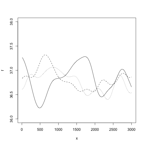
the variance of the likelihood model is set to 0.1. Samples from the prior Gaussian process can be drawn with

draw.sample(gp, 1:300*10, ep=0.000001)

Assuming we have the following observations

library(MASS)

xp <- beav1$time
yp <- beav1$temp

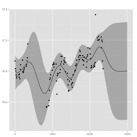
we may compute the posterior Gaussian processs with

gp <- posterior(gp, xp, yp)

The posterior distribution can be summarized and visualized at locations x with

x <- 1:300*10

summarize(gp, x)

plot(gp, x)

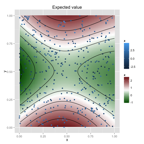
Data with higher-dimensional covariantes can be analysed in the same way, e.g. for two dimensions

np <- 400
xp <- cbind(x1 = runif(np), x2 = runif(np))
yp <- sin(pi*xp[,1]) + cos(2*pi*xp[,2]) + rnorm(np, 0, 1)

gp <- new.gp(0.5, kernel.squared.exponential(0.5, 1), dim=2)
gp <- posterior(gp, xp, yp, 1)

x  <- as.matrix(expand.grid(x = 1:100/100, y = 1:100/100))
plot(gp, x, plot.scatter=TRUE, plot.variance=FALSE)

Kernel functions

Name	Constructor	Parameters
Linear	kernel.linear	variance_0, variance, c (offset)
Squared exponential	kernel.squared.exponential	l, variance
Gamma exponential	kernel.gamma.exponential	l, variance, gamma
Periodic	kernel.periodic	l, variance, p (periodicity)
Locally periodic	kernel.locally.periodic	l, variance, p (periodicity)
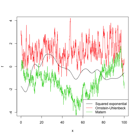
Ornstein-Uhlenbeck	kernel.ornstein.uhlenbeck	l, variance
Matern	kernel.matern	l, variance, nu
Combined kernel	kernel.combined	k1, k2, ..., kn (kernel functions)

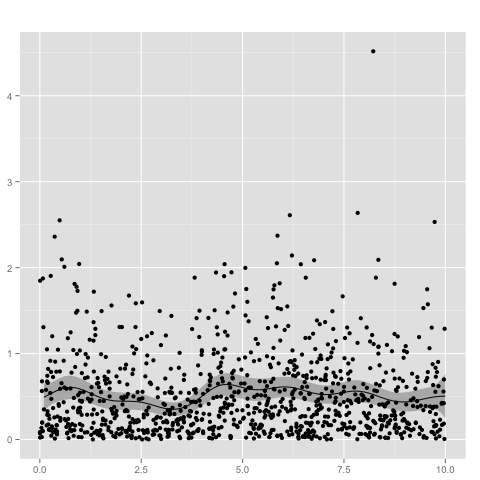
Likelihood models and link functions

Gamma likelihood model

The following example creates a Gaussian process with gamma likelihood. Since the domain of the gamma distribution is the positive reals, we need a link function, such as the logistic function, to transform the process.

gp <- new.gp(1.0, kernel.squared.exponential(1.0, 5.0),
	     likelihood=new.likelihood("gamma", 1.0),
	     link=new.link("logistic"))

The shape of the gamma likelihood is set to 1.0, whereas the mean is determined by the Gaussian process. Given the observations

n  <- 1000
xp <- 10*runif(n)
yp <- rgamma(n, 1, 2)

we obtain the posterior distribution with

# add some tiny noise to the diagonal for numerical stability
gp <- posterior(gp, xp, yp, ep=0.01, verbose=TRUE)
summarize(gp, 0:10/5)

plot(gp, 1:100/10)

Binomial likelihood

The probit link function can be used for binomial observations. In this case there is no specific likelihood model needed.

gp <- new.gp(0.5, kernel.squared.exponential(1, 0.25),
	     likelihood=NULL,
	     link=new.link("probit"))

The observations are given by

xp <- c(1,2,3,4)
yp <- matrix(0, 4, 2)
yp[1,] <- c(2, 14)
yp[2,] <- c(4, 12)
yp[3,] <- c(7, 10)
yp[4,] <- c(15, 8)

where xp is the locations of the observations and yp contains the count statistics (i.e. number of heads and tails).

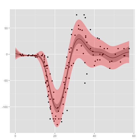
Heteroscedastic Gaussian process

Heteroscedasticity can be modeled with a second Gaussian process for the variance of the likelihood model. An example is given by

gp <- new.gp.heteroscedastic(
	new.gp( 0.0, kernel.squared.exponential(4, 100)),
	new.gp(10.0, kernel.squared.exponential(4,  10),
	       likelihood=new.likelihood("gamma", 1),
	       link=new.link("logistic")),
	transform     = sqrt,
	transform.inv = function(x) x^2)

where the second Gaussian process uses a gamma likelihood model in combination with a logistic link function. The empirical variances are transformed by taking the square root. Testing the model on the mcycle data set

data("mcycle", package = "MASS")

gp <- posterior(gp, mcycle$times, mcycle$accel, 0.00001,
                step = 0.1,
                epsilon = 0.000001,
                verbose=T)

gives the following result

Robust regression with heavy-tailed distributions

Heavy-tailed distributions, such as Student's t-distribution, are useful for modeling data that include outliers. Rasmussen's mode finding (a stabilized Newton's method, originally implemented in GPML) can be used for performing inference with Student's-t likelihood, which can be used for robust regression. Let us first generate a corrupted sin wave by

makeCorruptedSin <- function(x, basenoise, number_of_corruption, corruptionwidth){
        y_clean = sin(x)
        y = y_clean + rnorm(length(x),sd = basenoise)
        corruption_points = floor(runif(min=1, max=length(x),n = number_of_corruption))
        for (index in corruption_points){
            y[[index]] = y[[index]] + runif(min=-corruptionwidth, max=corruptionwidth, n = 1)
        }
        return(y)
}
    
x = seq(from=-3.14, to=3.14, by=0.1)
y = makeCorruptedSin(x, basenoise = 0.1, number_of_corruption = 25, corruptionwidth = 4)

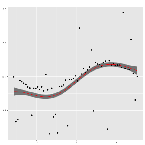
on which a Gaussian process with a Gaussian likelihood model

gp_n <- new.gp(0, kernel.squared.exponential(2, 2),
likelihood=new.likelihood("normal", 0.1))
gp_n <- posterior(gp_n, x, y)
plot(gp_n,x)

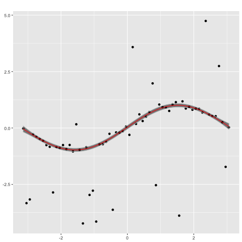
performs poorly. In contrast, a Gaussian process with a Student's t likelihood

gp_t <- new.gp(0, kernel.squared.exponential(2, 2),
         likelihood=new.likelihood("t", 2.1, 0.1))
gp_t <- posterior(gp_t, x, y, ep= 0.00000001, epsilon = 0.000001,
                verbose = TRUE, modefinding='rasmussen')
plot(gp_t,x)

captures the ground truth well.

pbenner / gp.regression