For encoding model of paper: Decoding and encoding models reveal the role of mental simulation in the brain representation of meaning

Requirement

python3.+
scikit-learn==0.22.0

METASEMA dataset

words: Spanish, 18 living words (i.e. cat, dog etc) and 18 nonliving words (i.e. mirror, knife etc)
task: read (shallow processing) or think of related features (deep processing)
3T MRI
27 subjects
15 ROIs

Goals

cross-validate standard encoding models using features extracted by word embedding models and computer vision models
compare the model performance among models use different features extracted by different word embedding models and computer vision models

Encoding Model Pipeline

clf             = linear_model.Ridge(
                  alpha        = 1e2,  # L2 penalty, higher means more regularization
                  normalize    = True, # normalize within each batch of feeding of the input data
                  random_state = 12345,# random seeding for reproducibility
)
X # feature representation matrix (n_samples x n_features)
y # BOLD signals                  (n_samples x n_voxels)
cv # cross validation method (indices)

scorer = make_scorer(r2_score,multioutput = "raw_values")

results = cross_validate(clf,X,y,cv = cv, scoring = scorer,) # need to write a customized for-loop for cross validation due to the specify requirement of the scorer
scores = results["test_score"]

Computing RDM

feature_representations # n_word x n_features
# subtract the mean of each "word" but not standardize it, or normalize each row to its unit vector form.
RDM = distance.squareform(distance.pdist(feature_representations - feature_representations.mean(1).reshape(-1,1),
                           metric = 'cosine',))
# fill NaNs for plotting
np.fill_diagonal(RDM,np.nan)

Results

Average Variance Explained

The average variance explained by the computer vision (VGG19, Densent169, MobilenetV2) and the word embedding (Fast Text, GloVe, Word2Vec) models, averaging across 27 subjects. The error-bars represent 95% confidence interval of a bootstrapping of 1000 iterations.

Difference between Computer Vision models and Word Embedding modles

Differences between computer vision and word embedding models in variance explained. Computer vision models significantly explained more variance of the BOLD response compared to word embedding models. All one-sample t-tests against zero difference between models were significant and FDR corrected for multiple comparisons.

The difference between CV and WE model contrasted between Shallow and Deep Processing conditions

Overall difference between Word Embedding and Computer Vision models per ROI (* FDR corrected for multiple comparisons). We found that the advantage of computer vision models over word embeddings models was higher in the deep processing condition relative to the shallow processing in PCG, PHG, and POP, while the opposite pattern was observed in FFG, IPL, and ITL

Number of positive voxel explained by the two models

The number of positive variance explained voxels for computer vision models and word embedding models. ROIs are color-coded and conditions are coded in different markers.

The difference of the number of positive variance explained voxels between computer vision models and word embedding models for each ROI and condition. *: p < 0.05, **: p < 0.01, ***: p < 0.0001.

Voxel-wise scores by the two models

Variance explained of individual voxels for all ROIs and conditions. ROIs are color-coded and conditions are coded in different makers. Particularly, voxels that cannot be positively explained by either the computer vision nor the word embedding models are shown by black circles. A few (~100 voxels for all subjects, ROIs, and conditions) that have extreme negative varience explained are not shown on the figure.

The posterior probability of computer vision models explain more variance than the word embedding models for a given voxel in a given ROI and condition. A prior probability of computer vision models explain more variance than the word embedding models was given by Beta(2, 2). This prior is centered at 0.5 and is lower for all other values. For a given ROI and condition, a voxel is better explained by the computer vision models was labeled “1” while “0” if vis versa. The posterior probability was computed by multiplying the prior probability and the likelihood of “1”. The posterior was normalized by divided its vector norm before reporting. θ: probability of computer vision models explain more variance than the word embedding models. The dotted line represents the average of initial prior probability, which means a naive belief that computer vision and word embedding models explain the same amount of variance for a given voxel.

Word Embedding Models in Spanish

source: Tommaso Teofili August 17, 2018

# for example, load fast test model in memory
fasttext_link: http://dcc.uchile.cl/~jperez/word-embeddings/fasttext-sbwc.vec.gz
fasttest_model = gensim.models.keyedvectors.KeyedVectors.load_word2vec_format(fasttext_downloaded_file_name)
for word in words:
    word_vector_representation = fasttest_model.get_vector(word)

Word vector (From Introduction to Word Vectors)

FastText, now supports 157 languages

@Article{bojanowski2016a,
  title={Enriching word vectors with subword information},
  author={Bojanowski, Piotr and Grave, Edouard and Joulin, Armand and Mikolov, Tomas},
  journal={Transactions of the Association for Computational Linguistics},
  volume={5},
  pages={135--146},
  year={2017},
  publisher={MIT Press}
}

Facebook AI Research lab
efficient learning for text classification
hierarchical classifier
Huffman algorithm to build the tree --> depth of frequent words is smaller than for infrequent ones
bag of words (BOW) -- ignore the word order
ngrams
represntational space = 300

GloVe

@CONFERENCE{Pennnigton2014a,
  title={Glove: Global vectors for word representation},
  author={Pennington, Jeffrey and Socher, Richard and Manning, Christopher},
  booktitle={Proceedings of the 2014 conference on empirical methods in natural language processing (\uppercase{EMNLP})},
  pages={1532--1543},
  year={2014}
}

Stanford
nearest neighbors
linear substructures
non-zero entries of a global word-word co-occurrence matrix
representational space = 300

Word2Vec - the 2013 paper

@inproceedings{mikolov2013a,
  title={Distributed representations of words and phrases and their compositionality},
  author={Mikolov, Tomas and Sutskever, Ilya and Chen, Kai and Corrado, Greg S and Dean, Jeff},
  booktitle={Advances in neural information processing systems},
  pages={3111--3119},
  year={2013}
}

skip-gram model with negative-sampling
minimum word frequency is 5
negative sampling at 20
273 most common words were downsampled
representational space = 300

Computer Vision Models

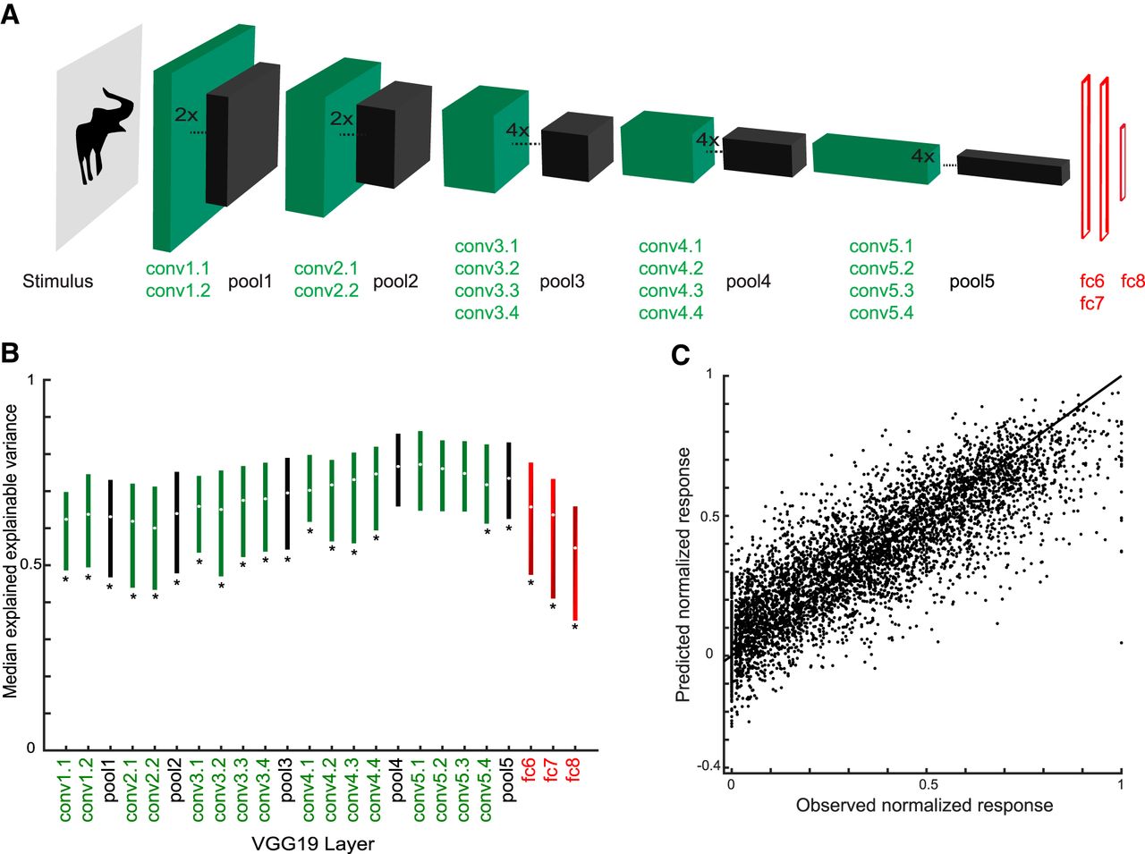
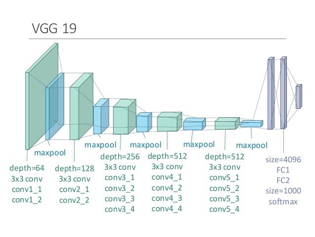
VGG19

@article{simonyan2014very,
  title={Very deep convolutional networks for large-scale image recognition},
  author={Simonyan, Karen and Zisserman, Andrew},
  journal={arXiv preprint arXiv:1409.1556},
  year={2014}
}

small convolution filters (3 x 3)
well-generalisible feature representations
representational space = 512

source: Kalfas et al., 2017

source: Yang et al., 2018

DenseNet121

@inproceedings{huang2017densely,
  title={Densely connected convolutional networks},
  author={Huang, Gao and Liu, Zhuang and Van Der Maaten, Laurens and Weinberger, Kilian Q},
  booktitle={Proceedings of the IEEE conference on computer vision and pattern recognition},
  pages={4700--4708},
  year={2017}
}

Each layer is receiving a “collective knowledge” from all preceding layers
The error signal can be easily propagated to earlier layers more directly. This is a kind of implicit deep supervision as earlier layers can get direct supervision from the final classification layer.
DenseNet performs well when training data is insufficient
representational space = 1028

source: Tsang, blog Nov 25, 2018

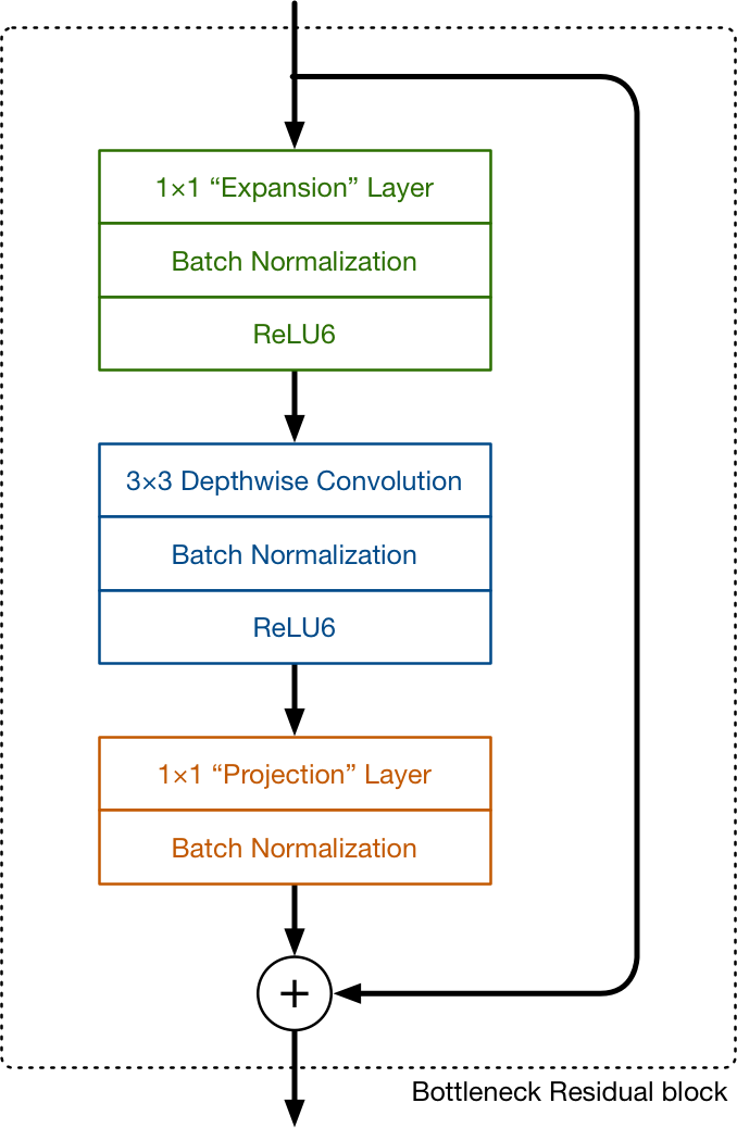
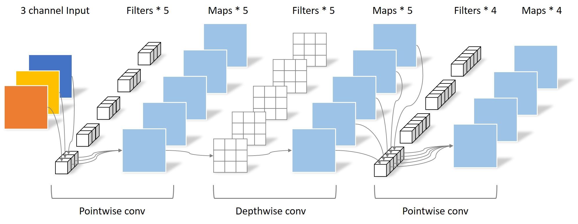
MobileNet_V2

@article{howard2017mobilenets,
  title={Mobilenets: Efficient convolutional neural networks for mobile vision applications},
  author={Howard, Andrew G and Zhu, Menglong and Chen, Bo and Kalenichenko, Dmitry and Wang, Weijun and Weyand, Tobias and Andreetto, Marco and Adam, Hartwig},
  journal={arXiv preprint arXiv:1704.04861},
  year={2017}
}