navining / cuda-raytracing

GPU acceleration of smallpt with CUDA. Obtain an acceleration of >35x comparing to the original CPU-parallelized code with OpenMP

GPU Acceleration of Ray Tracing with CUDA

Resources

RAI: The RAI client allows one to interact with a cluster of machine to submit and evaluate code.

Nvidia Performance Tools: NVIDIA Nsight Systems and Nsight Compute

Application

Ray Tracing

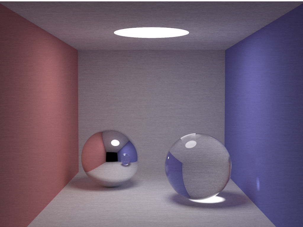
Ray tracing is a rendering technique widely used in computer graphics. In short, the principle of ray tracing is to trace the path of the light through each pixel, and simulate how the light beam encounters an object. Unlike rasterization technique which focuses on the realistic geometry of objects, ray tracing focuses on the simulation of light transport, where each ray is computational independent. This feature makes ray tracing suitable for a basic level of parallelization.

Potential Parallelism

Due to the characteristics of ray tracing algorithms, it is straightforward to convert the serial code into a parallel one, and the given code already implements a CPU-based parallel approach using OpenMP, where each image row runs in parallel. For the GPU parallel approach, we can use two-dimensional thread blocks and grids, in which each thread does computation for one pixel or a block of subpixels.

However, because of the divergence of ray paths, the computational workload of each pixel is different. Thus it is hard to achieve high utilization and low overhead under parallelization. Therefore, computation uniformity and work balance should be taken care of to optimize the performance.

Background

Currently there are many available codes to generate images using ray tracing algorithms, which can run on CPU or GPU in single or multi-thread methods. Existing CPU-based parallel approaches include dynamic scheduling and shared memory multiprocessing using OpenMP.

For GPU-based parallelism, there are various papers on this topic that target specific algorithms or data structures that can be used in ray tracing and implement new optimized structures suitable for GPU computing. In 2018, the announcements of NVIDIA’s new Turing GPUs, RTX technology spurred a renewed interest in ray tracing. NVIDIA gave a thorough walk through of translating C++ code to CUDA that results in a 10x or more speed improvement in their book Ray Tracing in One Weekend [1].

After doing some research online, we find some links/implementations that could be useful for our next step, listed in references.

References

[1] Allen, R. (2019, June 4). Accelerated Ray Tracing in One Weekend in CUDA. Retrieved May 12, 2020, from https://devblogs.nvidia.com/accelerated-ray-tracing-cuda/

[2] Razian S. A., Mohammadi H. M., “Optimizing Raytracing Algorithm Using CUDA,” Italian Journal of Science & Engineering, vol. 1, no. 3, pp. 167–178, 2017

[3] J, M., & Christiansen, M. (1958, May 1). raytracing with CUDA. Retrieved May 12, 2020, from https://stackoverflow.com/questions/39473/raytracing-with-cuda

[4] J.-C. Nebel. A New Parallel Algorithm Provided by a Computation Time Model, Eurographics Workshop on Parallel Graphics and Visualisation, 24–25 September 1998, Rennes, France.

[5] Chalmers, A., Davis, T., & Reinhard, E. (2002). Practical parallel rendering . Natick, MA.: AK Peters.

[6] Aila, T., and Laine, S. 2009. Understanding the efficiency of ray traversal on GPUs. In Proc. High Performance Graphics 2009 , 145--149.

Implementation

Overall Parallel Strategy

Our parallel strategy for ray tracing is quite straightforward: just let each thread do computation for one pixel. First, we developed functions to read the scene from an external file (“input.txt” by default) instead of hardcoding. The spheres are then saved in a host array. Memory for spheres and the output image is allocated on the device and copied from the host. Second, we set the grid dimension and block dimension, using 2-dimensional thread blocks to cover the whole image, where each thread does its own calculation for one pixel. Then kernel render() is executed where ray tracing of multiple samples in one pixel is conducted.

There are a couple of other modifications we made in order to have our code running properly, including but not limited to:

1. Modify necessary functions as __device__ so they can be called from the kernel. 2. Switch from recursion to iteration for function radiance() and limit the iteration depth to 10 since CUDA has a limitation in recursion depth of the kernel. A iteration version is much easier to debug and reduce function call overhead.
2. Use curand() instead of erand48() as the random number generator. curand() provides simple and efficient generation of high-quality pseudo-random numbers, which is sufficient in this project.

After the kernel execution, memory is copied back from device to host, and the image is written into an PPM file “image-cuda.ppm”.

Resulting Images

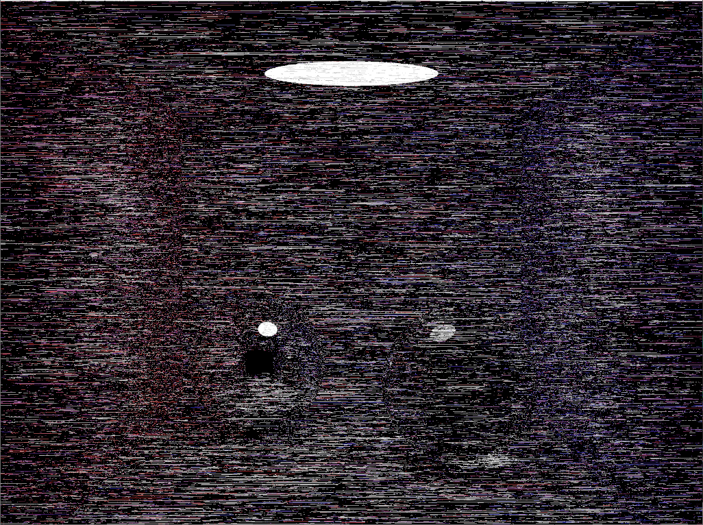
The parallel code can build and run on the server with RAI. The command to run the program is ./cu_smallpt <spp> <filename> . The following images were obtained with different samples per pixel.

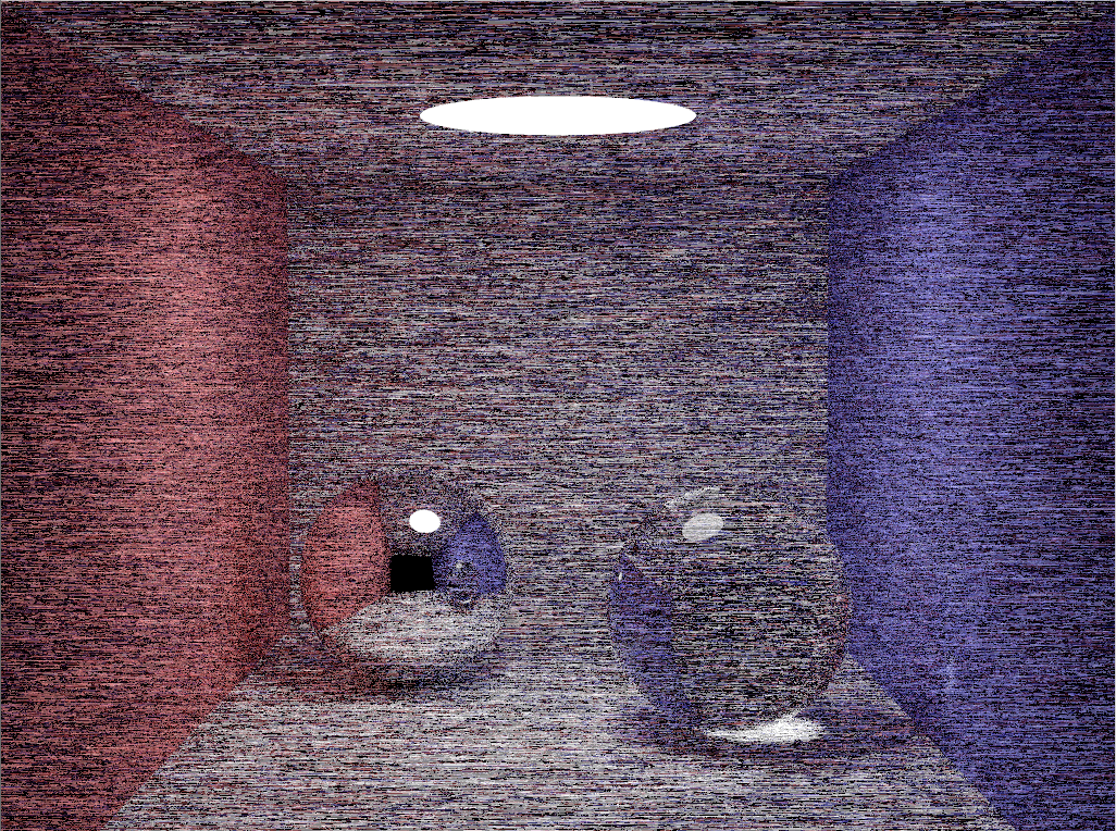
spp = 8	spp = 40
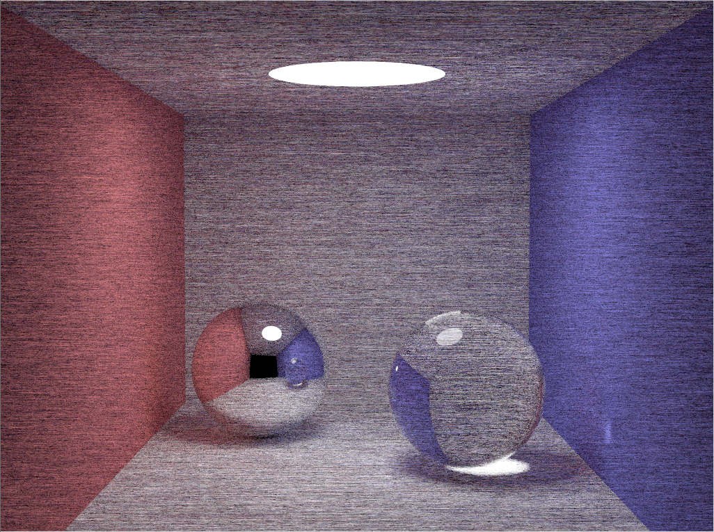
spp = 200	spp = 1000
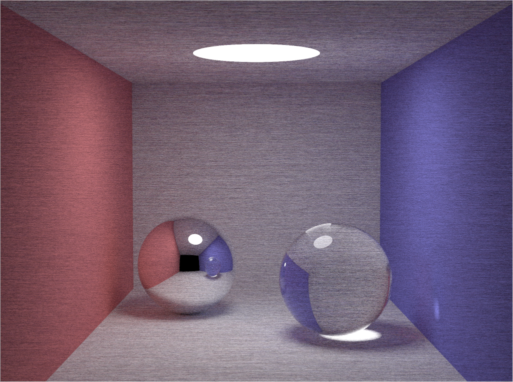
spp = 2000	spp = 5000

Performance Metrics: CPU (with OpenMP) vs. GPU

Here we compare our CUDA parallel version with the given CPU code using OpenMP parallelization.

Time (s)
spp	8	40	200	1000	2000	5000
CPU	0.99	4.24	20.00	98.58	201.15	510.22
GPU	0.68	0.83	1.30	3.50	6.32	14.63
Speedup	1.46	5.11	15.38	28.17	31.83	34.87

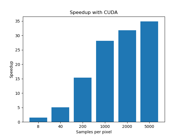
As we can see, GPU parallelization with CUDA achieves a great speedup in execution time, which initially proved the correctness of our parallelization approach.

Optimization

The parallel code is then optimized to achieve quicker execution time and lower Mean Squared Error (by comparing pixels with the target image). In this report, we will explain three optimizations in detail, but we also tried more methods that had no significant impact on the performance. The three optimizations we eventually used are : optimization of iteration code , optimization by lowering precision, and optimization by altering block size. All of these methods working together successfully helped us to meet the goal of less than 5 seconds for an MSE less than to 52.

Baseline Performance Analysis

The baseline CUDA version code is run under spp = 1000, and NVIDIA Nsight Compute is used for profiling.

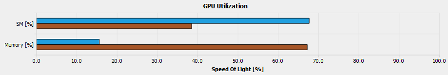
GPU Speed of Light

Time (s)	3.03
SoL SM (%)	38.48
SoL Memory (%)	67.18

After analyzing the utilization for compute and memory resources of the GPU, we can clearly see that memory is more heavily utilized than Compute. Therefore, a good optimization approach is to improve warp utilization or to reduce memory throughput.

Memory Workload

Memory Throughput (GB/s)	437.63
Global Load Cached	11.57G
Local Load Cached	4.89G
Shared Load	0
L1 Hit Rate (%)	64.13

Memory throughput is heavy here. Although most of the global memory access has been cached, there is still a huge amount of uncached local memory access. We should be able to further improve L1 Hit Rate by optimizing local load and store.

Scheduler Statistics

Theoretical Warps / Scheduler	16
Active Warps / Scheduler	3.91
Eligible Warps / Scheduler	0.29
Issued Warps / Scheduler	0.22

The size of warps should be 16 theoretically, but only 3.91 of them are active. Work imbalance of warps could be the main reason. There is still room for further optimization.

Warp State Statistics

Warp Cycles per Issued Instruction	17.42
Stall No Instructions	10.95
Stall Wait	3.14

On average each warp of this kernel spends 10.9 cycles being stalled due to not having the next instruction fetched yet. This represents about 62.8% of the total average of 17.4 cycles between issuing two instructions. A high number of warps not having an instruction fetched is typical for very short kernels with less than one full wave of work in the grid. Further improvement of warps utilization is needed.

Launch Statistics & Occupancy

Theoretical Occupancy (%)	25
Th. Active Warps per SM	16
Achieved Occupancy (%)	24.58
Waves per SM	19.20
Registers Per Thread	110

Theoretical occupancy is only a quarter due to the large amount of registers used by each thread. Resources can be better utilized if we can reduce register consumption.

Optimization 1 Optimizing Iteration Code

In our previous attempt, we converted the recursion in Radiance() function to iteration by using a stack to keep track of the variables and set a hard iteration limit. In the revised code, we removed the limit on iteration and removed the stack. Instead, we update two variables: accumulated color and accumulated reflectance.

	Baseline	With Optimization 1	Improvement (%)
Time (s)	3.03	2.74	-9.57%
SoL SM (%)	38.48	69.24	+79.93%
SoL Memory (%)	67.18	15.11	-77.51%

Memory Workload

	Baseline	With Optimization 1	Improvement (%)
Memory Throughput (GB/s)	437.63	0.015	-99.99%
L1 Hit Rate (%)	64.13	99.99	+55.91%

This approach hugely decreases the memory throughput. We eliminate all local memory loads and stores, thus nearly all memory access has been cached. In this case, shared memory is no longer needed as well.

Optimization 2 Double to Float

Double precision operations can be several times slower than single precision operations on some GPUs. We converted the type of some variables from double to float and marked constants in the code as ‘f’ to make the auto-conversion to double as late as possible.

	With Optimization 1	With Optimization 1&2	Improvement (%)
Time (s)	2.74	2.58	-5.84%
SoL SM (%)	69.24	65.79	-4.98%
SoL Memory (%)	15.11	15.03	-0.53%

Since the only change for Optimization 2 is lowering accuracy for couple operations, the final result meets our anticipation that the running time goes down a little bit while others stay the same.

Optimization 3 Optimizing Block Size

We changed the block size from 1616 to 3216. Larger block size ensures more warps available in each SM, therefore achieving better warp scheduling. Since the number of registers per SM could not exceed 65536 in current GPU, a larger block size won’t execute. Moreover, we make the block length able to be divisible by the image size in order to eliminate branch divergence.

	With Optimization 1&2	With Optimization 1,2&3	Improvement (%)
Time (s)	2.58	2.48	-3.88%
SoL SM (%)	65.79	67.66	+2.84%
SoL Memory (%)	15.03	15.57	+3.59%

This approach further shortens the time by 3.88%.

Results

Overall Optimization Results

GPU Speed of Light

	Baseline	With Optimization 1,2&3	Improvement (%)
Time (s)	3.03	2.48	-18.15%
SoL SM (%)	38.48	67.66	+75.84%
SoL Memory (%)	67.18	15.57	-76.82%

In all, we successfully optimized the usage of SM by 75.84%, and reduced the memory throughput by 76.82%. The improvement of time was not very significant compared with other factors, but it achieved a lower baseline.

Memory Workload

	Baseline	With Optimization 1,2&3	Improvement (%)
Memory Throughput (GB/s)	437.63	0.211	-99.95%
Global Load Cached	11.57G	19.88G	+71.80%
Local Load Cached	4.89G	0	-100%
Shared Load	0	0	0
Global Store	294K	294K	0
Local Store	4.09G	0.77G	-81.23%
L1 Hit Rate (%)	64.13	99.99	+55.91%

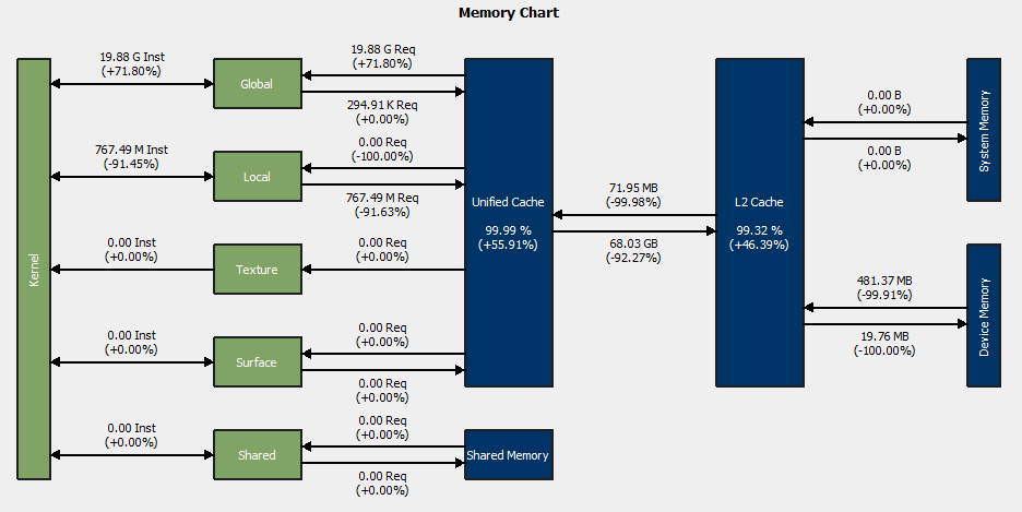
By converting 4.98G local load into global load, we could successfully obtain a L1 cache hit of 99.99% , thus decreasing memory throughput by 99.95% without using shared memory.

Scheduler Statistics

	Baseline	With Optimization 1,2&3	Improvement (%)
Theoretical Warps / Scheduler	16	16	0
Active Warps / Scheduler	3.91	3.92	+0.18%
Eligible Warps / Scheduler	0.29	0.73	+149.88%
Issued Warps / Scheduler	0.22	0.43	+93.31%

The improvement on eligible warps was significant by around 150%. There’s no obvious shift in active warps, and load balancing was still not optimal. It could be a limitation of the current parallel approach, since in the ray-tracing algorithm, the workload of each pixel (number of radiances) depends on the rendered scene itself.

Warp State Statistics

	Baseline	With Optimization 1,2&3	Improvement (%)
Warp Cycles per Issued Instruction	17.42	9.03	-48.17%
Stall No Instructions	10.95	2.19	-80.04%
Stall Wait	3.14	3.09	-1.80%

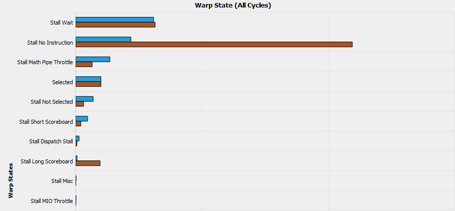
From the above graph, we can see that the warp stall was greatly eliminated, especially warp stall due to no instructions, which indicates a better utilization of warps.

Launch Statistics & Occupancy

	Baseline	With Optimization 1,2&3	Improvement (%)
Theoretical Occupancy (%)	25	25	0
Th. Active Warps per SM	16	16	0
Achieved Occupancy (%)	24.58	24.11	-1.89%
Waves per SM	19.20	19.20	0
Registers Per Thread	110	112	1.82%

After our optimization approaches, two extra registers are used per thread, which will slightly worsen the occupancy but has little effect on overall performance.

Final Performance Results

Execution Time

Here we compare our optimized CUDA parallel code with the given CPU code using OpenMP parallelization. As we can see, the optimized version has a better speedup with an average improvement close to 18%. A speedup of more than 35x is achieved with a large data set.

Time (s)
spp	8	40	200	1000	2000	5000
CPU	0.99	4.24	20.00	98.58	201.15	510.22
GPU	0.68	0.83	1.30	3.50	6.32	14.63
GPU w.o.	0.57	0.70	1.07	2.95	5.36	13.60
Speedup	1.74	6.06	18.69	33.42	37.53	37.52

Accuracy

Here we plot the mean squared error vs. the execution time. As we can see, with samples per pixel more than 1000 can the target image achieve a target MSE of 52. 1000 spp is pretty close to the criteria, so let’s say using 1100 samples per pixel is safe enough to pass the threshold with an execution time under 5 seconds.

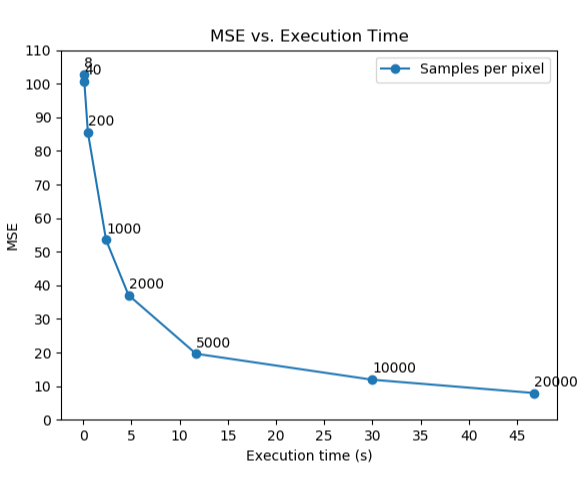
With 1100 samples per pixel, we obtained the final result with a MSE of 51.28 and an execution time of 3.09s.

Conclusions

From the speedup result of using CUDA for GPU parallelization, we realized the advantages of GPU over CPU in dense floating point arithmetic, for example image processing and matrix calculations. The architecture features of GPU makes it the best candidate for ray tracing acceleration.

Different from optimizations such as matrix multiplication, it could happen that some universal approval methods may not be useful under different scenarios. For example, using shared memory would not make a great difference in our project because memory bandwidth is not the bottleneck of performance. However, all of us finally admit that optimization is highly dependent on our algorithms as well.