Michael Jahn 2022-03-16
An Interface to Import and Modify SVG (XML) Graphic Files in R.
SVG is the primary choice for scalable, open-source graphic files. This packages provides a simple interface to import SVG graphic files in R, modify these in a programmatic way, and export the files again. The purpose of this package is to overlay scientific data on medium or large scale network representations, which is too laborious and time-consuming to do manually. SVG Graphics have to be drawn beforehand, for example using Inkscape. Objects (“nodes”) are than identified and modified using unique IDs/label in R. The fantastic Escher app follows a similar approach, where a metabolic network is first drawn on a canvas, and then used as a template to overlay metabolic, flux, gene expression or other data. Options to customize the metabolic maps are too restricted.
Package info:
- Maintainer: Michael Jahn, Science for Life Lab, Stockholm
- License: GPL-3
- Depends: R (>= 3.5.0)
- Imports:
methods,XML,dplyr
To install the package directly from github, use the following function
from the devtools package in your R session:
devtools::install_github("m-jahn/fluctuator")The first step is to create an SVG file depicting e.g. a metabolic
network. Inkscape is a free, open source software for vector images and
natively supports SVG. Every item (node) that is created gets a cryptic
label in Inkscape, such as path-123-456-0-1. All we need to do is to
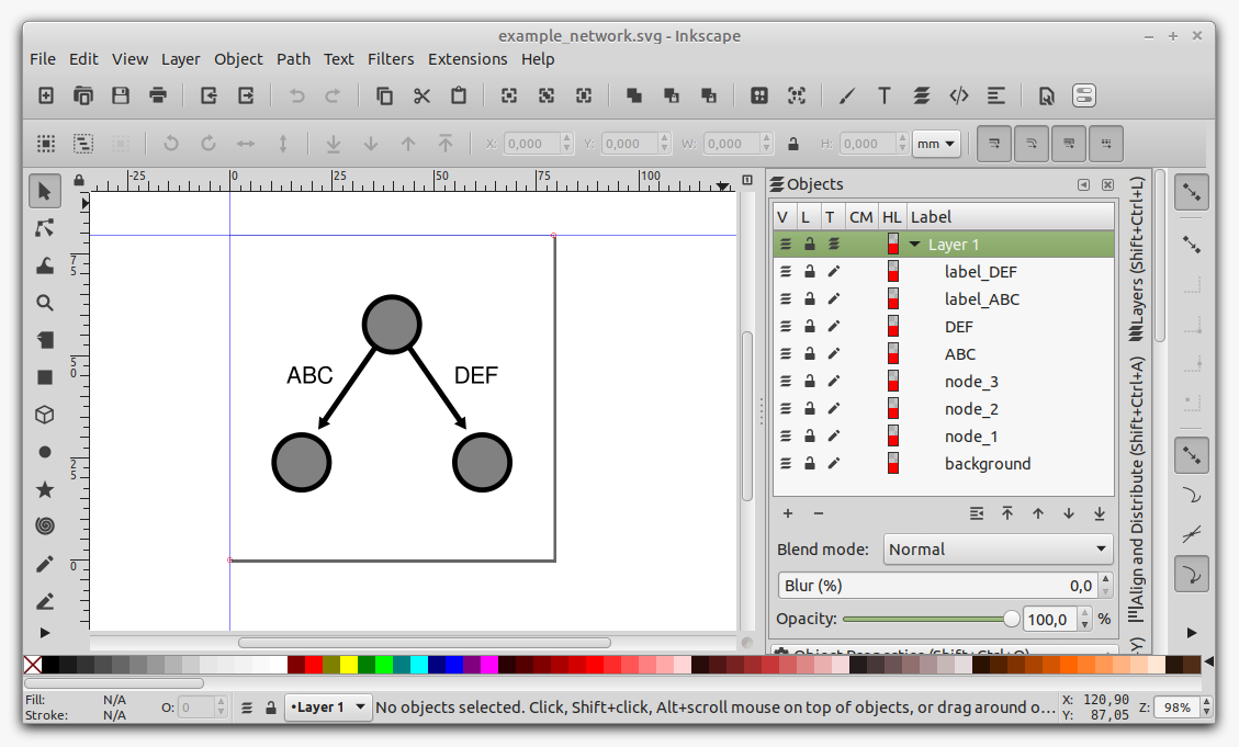
open the object dialog and change labels to more human readable names
(see picture). These are later used to identify objects in R. I
recommend using different prefixes for different types of objects, like
node_XYZ for the nodes of a network, and reaction_XYZ for
connections between nodes.
We can then import the SVG file in R using read_svg(). The resulting
object of class XMLsvg has two slots, the original XML structure and a
feature table with all graphical objects (nodes) and their attributes.
library(dplyr)
library(fluctuator)

# import example map
SVG <- read_svg("inst/extdata/example_network.svg")

# show class
class(SVG)
## [1] "XMLsvg"
## attr(,"package")
## [1] "fluctuator"
# access summary table of objects/nodes
head(SVG@summary)
## # A tibble: 6 × 23
## node_no id d style transform `connector-cur…` node_set label cx
## <chr> <chr> <chr> <chr> <chr> <chr> <chr> <chr> <chr>
## 1 1 path4920 M 5.… fill… scale(0.… 0 path <NA> <NA>
## 2 2 path4920-8 M 5.… fill… scale(0.… 0 path <NA> <NA>
## 3 3 path4770 M 52… fill… <NA> 0 path ABC <NA>
## 4 4 path4770-1 M 60… fill… <NA> 0 path DEF <NA>
## 5 5 path4747 <NA> colo… <NA> <NA> circle node… 56.4…
## 6 6 path4747-3 <NA> colo… <NA> <NA> circle node… 34.3…
## # … with 14 more variables: cy <chr>, r <chr>, stockid <chr>, orient <chr>,
## # refY <chr>, refX <chr>, isstock <chr>, space <chr>, x <chr>, y <chr>,
## # role <chr>, groupmode <chr>, width <chr>, height <chr>
We can search for certain nodes in the SVG and display their attributes. Note that nodes are objects, not to be confused with single points of a path.
get_attributes(SVG, node = "node_1", attr = c("label", "style"))## # A tibble: 1 × 2
## label style
## <chr> <chr>
## 1 node_1 color:#000000;clip-rule:nonzero;display:inline;overflow:visible;visibi…
get_attributes(SVG, node = "ABC", attr = c("label", "style"))## # A tibble: 1 × 2
## label style
## <chr> <chr>
## 1 ABC fill:#000000;fill-opacity:1;fill-rule:evenodd;stroke:#000000;stroke-wid…
The most important feature of this package is to change SVG attributes
using the set_attributes() function. The function takes four important
arguments: the name (label) of the node whose attributes should be
changed, and which corresponds to Inkscape object names. The attribute
that is supposed to be changed (e.g. style). And a pattern +
replacement that modifies the character value of the attribute.
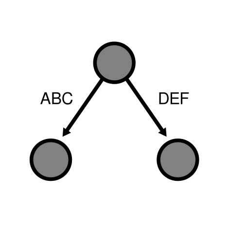
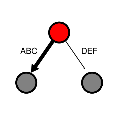
In this example we change the fill color of node_1 to red. Then we
also change the thickness of the two arrows (reactions) ABC and DEF.
SVG <- set_attributes(SVG, node = "node_1", attr = "style",
  pattern = "fill:#808080", replacement = "fill:#FF0000")

SVG <- set_attributes(SVG, node = c("ABC", "DEF"), attr = "style",
pattern = "stroke-width:1.32291663", replacement = c("stroke-width:2.5", "stroke-width:0.5"))Modified SVG files can be saved to disk using write_svg().
write_svg(SVG, file = "inst/extdata/example_network_mod.svg")| Original SVG | Modified SVG |
|---|---|
 |
 |
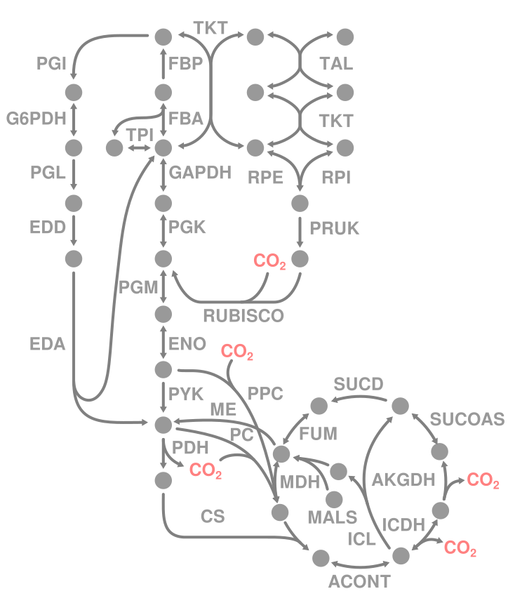
Let’s import a reduced network of the central carbon metabolism of the
bacterium Cupriavidus necator. We can inspect the Inkscape names of
all reactions in the summary table (column label).
SVG2 <- read_svg("inst/extdata/central_metabolism.svg")
head(SVG2@summary)
## # A tibble: 6 × 25
## node_no id d style transform `connector-cur…` node_set nodetypes label
## <chr> <chr> <chr> <chr> <chr> <chr> <chr> <chr> <chr>
## 1 1 path1… M 5.… fill… scale(0.… 0 path <NA> <NA>
## 2 2 path1… M 5.… fill… scale(-0… 0 path <NA> <NA>
## 3 3 path1… M 5.… fill… scale(0.… 0 path <NA> <NA>
## 4 4 path1… M 5.… fill… scale(0.… 0 path <NA> <NA>
## 5 5 path8… M 5.… fill… scale(0.… 0 path <NA> <NA>
## 6 6 path8… M 5.… fill… scale(0.… 0 path <NA> <NA>
## # … with 16 more variables: y <chr>, x <chr>, role <chr>, space <chr>,
## # stockid <chr>, orient <chr>, refY <chr>, refX <chr>, isstock <chr>,
## # collect <chr>, cx <chr>, cy <chr>, r <chr>, groupmode <chr>, width <chr>,
## # height <chr>
The network has objects for metabolites, reactions, and reaction text labels. We want to modify the thickness of arrows representing flux through reactions. We import a table with flux data matching the reactions in the SVG file.
data(metabolic_flux)
head(metabolic_flux)
## # A tibble: 6 × 3
## substrate reaction flux_mmol_gDCW_h
## <chr> <chr> <dbl>
## 1 formate ACONT 0.366
## 2 formate AKGDH 0
## 3 formate CS 0.366
## 4 formate EDA 0
## 5 formate EDD 0
## 6 formate ENO 3.98
Then we inspect the style of the nodes that we want to change, and find
the text bit for stroke-width.
get_attributes(SVG2, node = "GAPDH") %>% pull(style)## [1] "opacity:1;vector-effect:none;fill:none;fill-opacity:1;fill-rule:evenodd;stroke:#808080;stroke-width:0.34395832;stroke-linecap:round;stroke-linejoin:round;stroke-miterlimit:4;stroke-dasharray:none;stroke-dashoffset:0;stroke-opacity:1;marker-start:url(#marker11347);marker-end:url(#marker66490);enable-background:new"
As some reactions have very high flux and others no flux at all, we apply a square root transformation to the fluxes so that stroke width is more balanced.
metabolic_flux <- metabolic_flux %>%
  mutate(stroke_width = 0.5 + 0.2*sqrt(abs(flux_mmol_gDCW_h)))

SVG2 <- set_attributes(SVG2,
  node = metabolic_flux$reaction, attr = "style",
  pattern = "stroke-width:[0-9]+\\.[0-9]+",
  replacement = paste0("stroke-width:", metabolic_flux$stroke_width))
We can also change the color according to metabolic flux.
# make color palette
pal <- colorRampPalette(c("#ABABAB", "#009419", "#F0B000", "#FF4800"))(10)

metabolic_flux <- metabolic_flux %>%
  mutate(
    stroke_color = stroke_width %>% {1+(./max(.))*9} %>% round,
    stroke_color_rgb = pal[stroke_color])

SVG2 <- set_attributes(SVG2,
  node = metabolic_flux$reaction, attr = "style",
  pattern = "stroke:#808080",
  replacement = paste0("stroke:", metabolic_flux$stroke_color_rgb))
And for better look, reduce the size of the arrow heads. Arrow heads are
called marker in Inkscape SVG (note that node name attribute changed
to id). To modify size, we change the transform field of the marker
nodes. Needs to be done separately for start and end arrows.
SVG2 <- set_attributes(SVG2,
  node = grep("marker", SVG2@summary$id, value = TRUE),
  node_attr = "id",
  attr = "transform",
  pattern = "scale\\(0.2\\)",
  replacement = "scale(0.15)")

SVG2 <- set_attributes(SVG2,
  node = grep("marker", SVG2@summary$id, value = TRUE),
  node_attr = "id",
  attr = "transform",
  pattern = "scale\\(-0.2\\)",
  replacement = "scale(-0.15)")
Export the modified SVG file.
write_svg(SVG2, file = "inst/extdata/central_metabolism_mod.svg")## [1] "inst/extdata/central_metabolism_mod.svg"
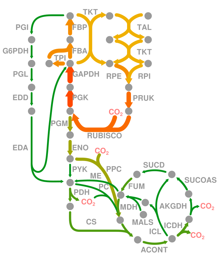
| Original SVG | SVG with overlaid fluxes |
|---|---|
 |
 |
Practically every object of the SVG files can be modified in R. Here is an (incomplete) list of modifications that can be useful when working with metabolic maps, or other scientific images that profit from overlaying numerical data.
Some reactions in the previous example are reversible, hence they have
arrows at the start and at the end. However, the flux in one particular
condition can only go in one direction. To visualize only forward or
only backward flux, we can remove arrow heads from selected reactions.
In the example below the marker-end:... string is removed for all
reactions with negative flux and the marker-start:... string for all
reactions with positive flux.
SVG2 <- set_attributes(SVG2,
  node = filter(metabolic_flux, flux_mmol_gDCW_h < 0)$reaction,
  attr = "style",
  pattern = "marker-end:url\\(#marker[0-9]*\\);",
  replacement = "")

SVG2 <- set_attributes(SVG2,
  node = filter(metabolic_flux, flux_mmol_gDCW_h >= 0)$reaction,
  attr = "style",
  pattern = "marker-start:url\\(#marker[0-9]*\\);",
  replacement = "")

write_svg(SVG2, file = "inst/extdata/central_metabolism_direction.svg")
## [1] "inst/extdata/central_metabolism_direction.svg"
| SVG with overlaid fluxes | SVG with correct directionality |
|---|---|
 |
 |
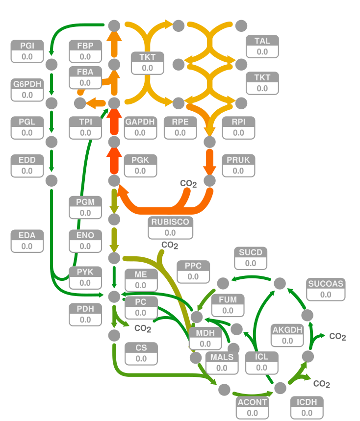
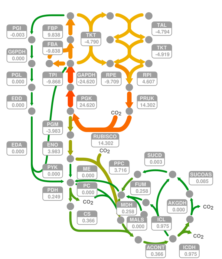
We can also change text fields in the SVG file and by these means add
numeric flux data. All we need is a template that has predefined text
fields, whose values are then changed using set_values(). Values are
different “fields” in XML files and therefore require an own
modification function. We can load a template map that has text fields
named value_REACTION. First we can inspect the current values using
get_values() analogously to get_attributes().
SVG3 <- read_svg("inst/extdata/central_metabolism_values.svg")
get_values(SVG3, node = c("value_ACONT", "value_AKGDH", "value_CS"))
## value_ACONT value_AKGDH value_CS
## "0.0" "0.0" "0.0"
Then we set new values.
SVG3 <- set_values(SVG3,
  node = paste0("value_", metabolic_flux$reaction),
  value = round(metabolic_flux$flux_mmol_gDCW_h, 3)
)

write_svg(SVG3, file = "inst/extdata/central_metabolism_values_filled.svg")
## [1] "inst/extdata/central_metabolism_values_filled.svg"
| SVG template for values | SVG with added flux values |
|---|---|
 |
 |


