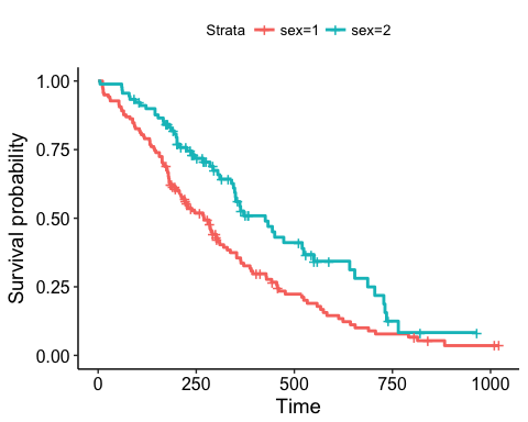
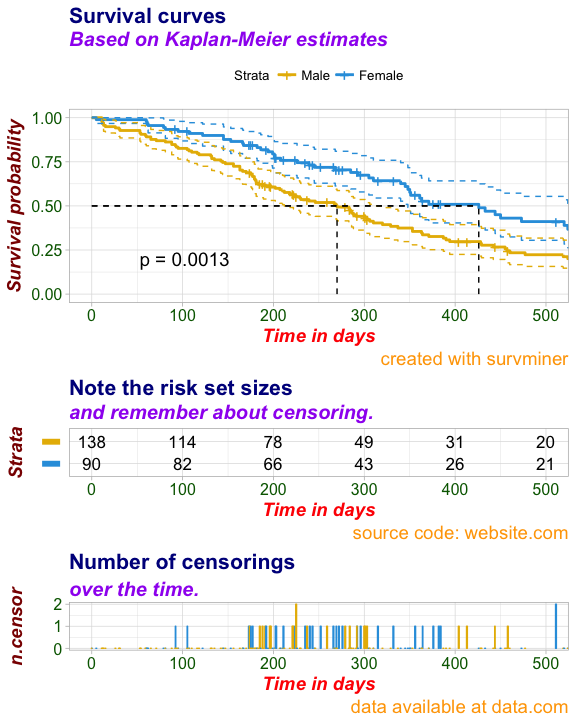
The survminer R package provides functions for facilitating survival analysis and visualization. The current version contains three main functions including:
-
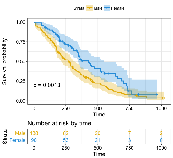
ggsurvplot(): Draws survival curves with the 'number at risk' table and 'censoring count plot'.
-
ggcoxzph(): Graphical test of proportional hazards.
-
ggcoxfunctional(): Displays graphs of continuous explanatory variable against martingale residuals of null cox proportional hazards model. It helps to properly choose the functional form of continuous variable in cox model.
Find out more at http://www.sthda.com/english/rpkgs/survminer/, and check out the documentation and usage examples of each of the functions in survminer package.
Install from CRAN as follow:
install.packages("survminer")Or, install the latest version from GitHub:
if(!require(devtools)) install.packages("devtools")
devtools::install_github("kassambara/survminer", build_vignettes = FALSE)
Load survminer:
library("survminer")
# Loading required package: ggplot2require("survival")
# Loading required package: survival
fit <- survfit(Surv(time, status) ~ sex, data = lung)ggsurvplot(fit)ggsurvplot(fit, size = 1, # change line size
palette = c("#E7B800", "#2E9FDF"), # custom color palettes
conf.int = TRUE, # Add confidence interval
pval = TRUE, # Add p-value
risk.table = TRUE, # Add risk table
risk.table.col = "strata", # Risk table color by groups
legend.labs = c("Male", "Female"), # Change legend labels
risk.table.height = 0.25, # Useful to change when you have multiple groups
ggtheme = theme_bw() # Change ggplot2 theme
)Note that, additional arguments are available to customize the main title, axis labels, the font style, axis limits, legends and the number at risk table.
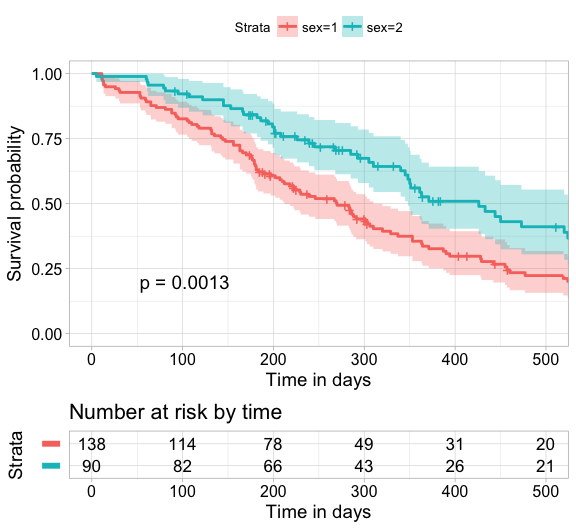
Focus on xlim and break.time.by parameters which do not change the calculations of estimates of survival surves. Also note risk.table.y.text.col = TRUE and risk.table.y.text = FALSE that provide bars instead of names in text annotations of the legend of risk table.
ggsurvplot(
   fit,                     # survfit object with calculated statistics.
   risk.table = TRUE,       # show risk table.
   pval = TRUE,             # show p-value of log-rank test.
   conf.int = TRUE,         # show confidence intervals for
                            # point estimates of survival curves.
   xlim = c(0,500),         # present narrower X axis, but not affect
                            # survival estimates.
   xlab = "Time in days",   # customize X axis label.
   break.time.by = 100,     # break X axis in time intervals by 500.
   ggtheme = theme_light(), # customize plot and risk table with a theme.
 risk.table.y.text.col = T, # colour risk table text annotations.
  risk.table.y.text = FALSE # show bars instead of names in text annotations
                            # in legend of risk table
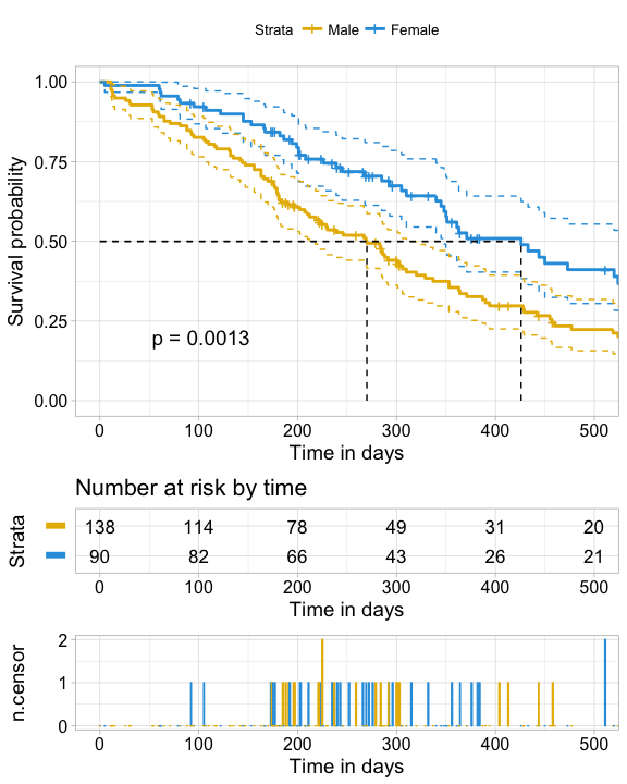
)ggsurvplot(
fit, # survfit object with calculated statistics.
risk.table = TRUE, # show risk table.
pval = TRUE, # show p-value of log-rank test.
conf.int = TRUE, # show confidence intervals for
# point estimates of survival curves.
xlim = c(0,500), # present narrower X axis, but not affect
# survival estimates.
xlab = "Time in days", # customize X axis label.
break.time.by = 100, # break X axis in time intervals by 500.
ggtheme = theme_light(), # customize plot and risk table with a theme.
risk.table.y.text.col = T,# colour risk table text annotations.
risk.table.y.text = FALSE,# show bars instead of names in text annotations
# in legend of risk table.
ncensor.plot = TRUE, # plot the number of censored subjects at time t
conf.int.style = "step", # customize style of confidence intervals
surv.median.line = "hv", # add the median survival pointer.
legend.labs =
c("Male", "Female"), # change legend labels.
palette =
c("#E7B800", "#2E9FDF") # custom color palettes.
)ggsurvplot(
fit, # survfit object with calculated statistics.
risk.table = TRUE, # show risk table.
pval = TRUE, # show p-value of log-rank test.
conf.int = TRUE, # show confidence intervals for
# point estimates of survival curves.
xlim = c(0,500), # present narrower X axis, but not affect
# survival estimates.
xlab = "Time in days", # customize X axis label.
break.time.by = 100, # break X axis in time intervals by 500.
ggtheme = theme_light(), # customize plot and risk table with a theme.
risk.table.y.text.col = T,# colour risk table text annotations.
risk.table.y.text = FALSE,# show bars instead of names in text annotations
# in legend of risk table.
ncensor.plot = TRUE, # plot the number of censored subjects at time t
conf.int.style = "step", # customize style of confidence intervals
surv.median.line = "hv", # add the median survival pointer.
legend.labs =
c("Male", "Female"), # change legend labels.
palette =
c("#E7B800", "#2E9FDF"),# custom color palettes.
main = "Survival curves", # specify the title of the plot
submain = "Based on Kaplan-Meier estimates", # the subtitle of the plot
caption = "created with survminer", # the caption of the plot
font.main = c(16, "bold", "darkblue"), # font for titles of the plot, the table and censor part
font.submain = c(15, "bold.italic", "purple"), # font for subtitles in the plot, the table and censor part
font.caption = c(14, "plain", "orange"), # font for captions in the plot, the table and censor part
font.x = c(14, "bold.italic", "red"), # font for x axises in the plot, the table and censor part
font.y = c(14, "bold.italic", "darkred"), # font for y axises in the plot, the table and censor part
font.tickslab = c(12, "plain", "darkgreen"), # font for ticklabs in the plot, the table and censor part
########## risk table #########,
risk.table.title = "Note the risk set sizes", # the title of the risk table
risk.table.subtitle = "and remember about censoring.", # the subtitle of the risk table
risk.table.caption = "source code: website.com", # the caption of the risk table
risk.table.height = 0.35, # the height of the risk table
########## ncensor plot ######
ncensor.plot.title = "Number of censorings", # as above but for the censoring plot
ncensor.plot.subtitle = "over the time.",
ncensor.plot.caption = "data available at data.com",
ncensor.plot.height = 0.35
)-
M. Kosiński. R-ADDICT January 2017. When You Went too Far with Survival Plots During the survminer 1st Anniversary
-
A. Kassambara. STHDA December 2016. Survival Analysis Basics: Curves and Logrank Tests
-
A. Kassambara. STHDA December 2016. Cox Proportional Hazards Model
-
A. Kassambara. STHDA December 2016. Cox Model Assumptions
-
M. Kosiński. R-ADDICT November 2016. Determine optimal cutpoints for numerical variables in survival plots
-
M. Kosiński. R-ADDICT May 2016. Survival plots have never been so informative
-
A. Kassambara. STHDA January 2016. survminer R package: Survival Data Analysis and Visualization.

