This repository is a python implementation of tabular-methods for reinforcement learning focusing on the dynamic programming and temporal difference methods presented in Reinforcement Learning, An Introduction. The following algorithms are implemented:
- Value Iteration: see page 67 of Reinforcement Learning, An Introduction
- Policy Iteration: see page 64 of Reinforcement Learning, An Introduction
- SARSA, on-policy TD control: see page 105 of Reinforcement Learning, An Introduction
- Q-Learning off-policy TD control: see page 107 of Reinforcement Learning, An Introduction
Notes:
- Tested for python >= 3.5
Table of Contents:
# clone repo
pip install -r requirements.txt
This describes the example found in examples/example_plot_gridworld.py which illustrates all the
functionality of the GridWorld class found in env/grid_world.py. It shows how to:
- Define the grid world size by specifying the number of rows and columns.
- Add a single start state.
- Add multiple goal states.
- Add obstructions such as walls, bad states and restart states.
- Define the rewards for the different types of states.
- Define the transition probabilities for the world.
The grid world is instantiated with the number of rows, number of columns, start state and goal states:
# specify world parameters
num_rows = 10
num_cols = 10
start_state = np.array([[0, 4]]) # shape (1, 2)
goal_states = np.array([[0, 9],
                        [2, 2],
                        [8, 7]]) # shape (n, 2)

gw = GridWorld(num_rows=num_rows,
               num_cols=num_cols,
               start_state=start_state,
               goal_states=goal_states)
Add obstructed states, bad states and restart states:
- Obstructed states: walls that prohibit the agent from entering that state.
- Bad states: states that incur a greater penalty than a normal step.
- Restart states: states that incur a high penalty and transition the agent back to the start state (but do not end the episode).
obstructions = np.array([[0,7],[1,1],[1,2],[1,3],[1,7],[2,1],[2,3],
                         [2,7],[3,1],[3,3],[3,5],[4,3],[4,5],[4,7],
                         [5,3],[5,7],[5,9],[6,3],[6,9],[7,1],[7,6],
                         [7,7],[7,8],[7,9],[8,1],[8,5],[8,6],[9,1]]) # shape (n, 2)
bad_states = np.array([[1,9],
                       [4,2],
                       [4,4],
                       [7,5],
                       [9,9]])      # shape (n, 2)
restart_states = np.array([[3,7],
                           [8,2]])  # shape (n, 2)

gw.add_obstructions(obstructed_states=obstructions,
                    bad_states=bad_states,
                    restart_states=restart_states)
Define the rewards for the obstructions:
gw.add_rewards(step_reward=-1,
               goal_reward=10,
               bad_state_reward=-6,
               restart_state_reward=-100)
Add transition probabilities to the grid world.
p_good_transition is the probability that the agent successfully executes the intended action. The action is then incorrectly executed with probability 1 - p_good_transition and in tis case the agent transitions to the left of the intended transition with probability (1 - p_good_transition) * bias and to the right with probability (1 - p_good_transition) * (1 - bias).
gw.add_transition_probability(p_good_transition=0.7,
                              bias=0.5)
Finally, add a discount to the world and create the model.
gw.add_discount(discount=0.9)
model = gw.create_gridworld()
The created grid world can be viewed with the plot_gridworld function in utils/plots.
plot_gridworld(model, title="Test world")
Here the created grid world is solved through the use of the dynamic programming method
value iteration (from examples/example_value_iteration.py). See also
examples/example_policy_iteration.py for the equivalent solution via policy iteration.
Apply value iteration to the grid world:
# solve with value iteration
value_function, policy = value_iteration(model, maxiter=100)

# plot the results
plot_gridworld(model, value_function=value_function, policy=policy, title="Value iteration")
This example describes the code found in examples/example_sarsa.py and examples/example_qlearning.py
which use SARSA and Q-Learning to replicate the solution to the classic cliff walk environment on page 108 of
Sutton's book.
The cliff walk environment is created with the code:
# specify world parameters
num_rows = 4
num_cols = 12
restart_states = np.array([[3,1],[3,2],[3,3],[3,4],[3,5],
                           [3,6],[3,7],[3,8],[3,9],[3,10]])
start_state = np.array([[3,0]])
goal_states = np.array([[3,11]])

# create model
gw = GridWorld(num_rows=num_rows,
               num_cols=num_cols,
               start_state=start_state,
               goal_states=goal_states)
gw.add_obstructions(restart_states=restart_states)
gw.add_rewards(step_reward=-1,
               goal_reward=10,
               restart_state_reward=-100)
gw.add_transition_probability(p_good_transition=1,
                              bias=0)
gw.add_discount(discount=0.9)
model = gw.create_gridworld()

# plot the world
plot_gridworld(model, title="Cliff Walk")
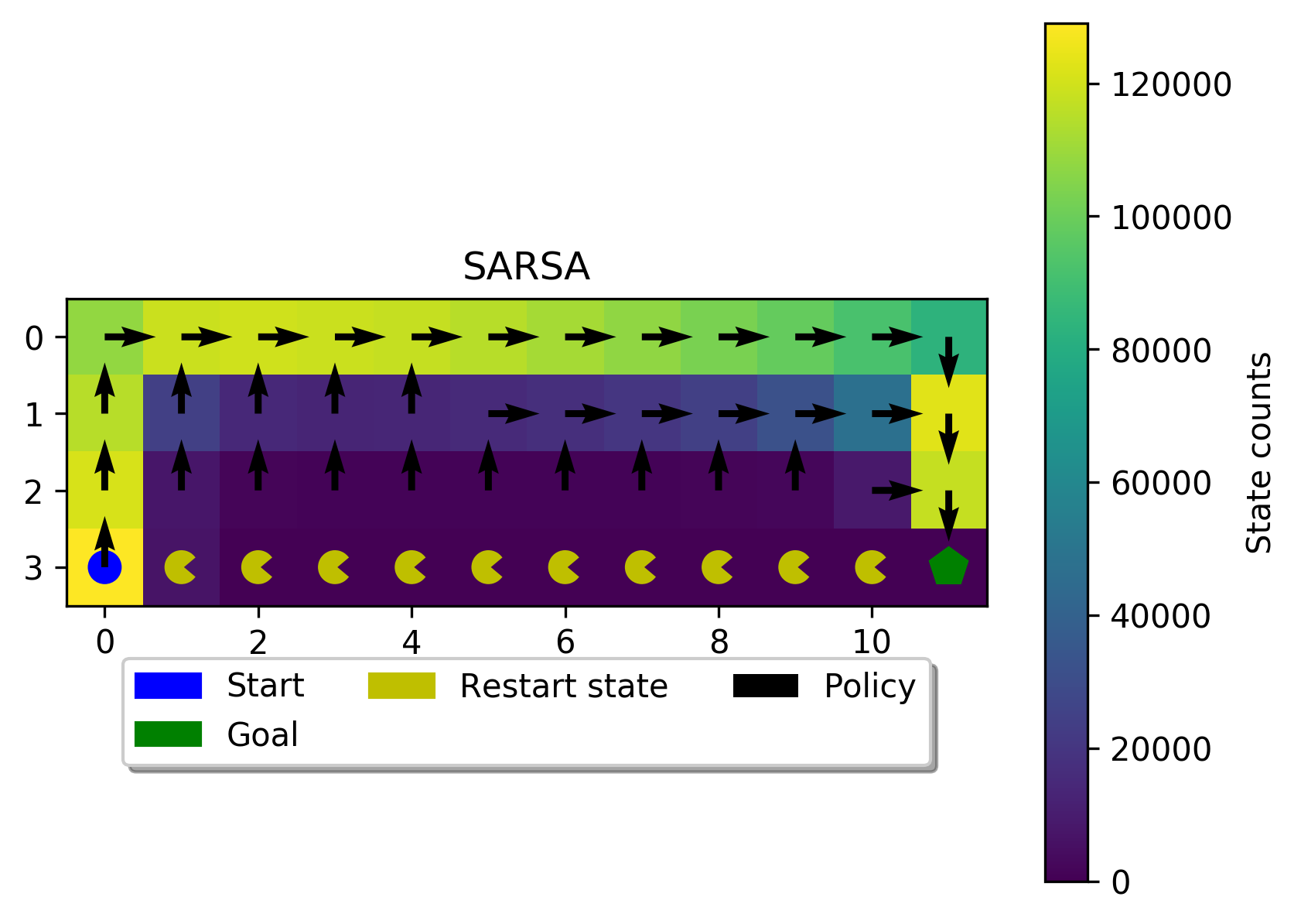
Solve the cliff walk with the on-policy temporal difference control method SARSA and plot the results.
SARSA returns three values, the q_function, the policy and the state_counts. Here the policy and the
state_counts are passed to plot_gridworld so that the path most frequently used by the agent is shown.
However, the q_function can be passed instead to show the q_function values on the plot as was done with
the dynamic programming examples.
# solve with SARSA
q_function, pi, state_counts = sarsa(model, alpha=0.1, epsilon=0.2, maxiter=100, maxeps=100000)

# plot the results
plot_gridworld(model, policy=pi, state_counts=state_counts, title="SARSA")
Solve the cliff walk with the off-policy temporal difference control method Q-Learning and plot the results.
# solve with Q-Learning
q_function, pi, state_counts = qlearning(model, alpha=0.9, epsilon=0.2, maxiter=100, maxeps=10000)

# plot the results
plot_gridworld(model, policy=pi, state_counts=state_counts, title="Q-Learning", path=path)
From the plots, it is clear that the SARSA agent learns a conservative solution to the cliff walk and shows preference for the path furthest away from the cliff edge. In contrast, the Q-Learning agent learns the riskier path along the cliff edge.
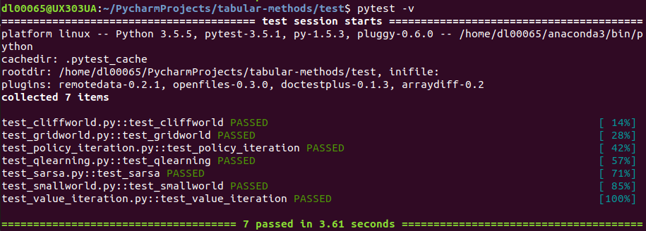
Testing setup with pytest (requires installation). Should you want to check version
compatibility or make changes, you can check that original tabular-methods functionality remains unaffected by
executing pytest -v in the test directory. You should see the following:


