konstantinklemmer / sxl

SXL: Spatially explicit learning of geographic processes with auxiliary tasks

SXL - Spatially explicit learning of geographic processes with auxiliary tasks

This repository provides complementary code and data for our paper "Auxiliary-task learning for geographic data with autoregressive embeddings" (Long version, Short version)

With SXL, models learn spatial autocorrelation patterns in the data (at different resolutions) alongside the primary predictive or generative modeling task. These auxiliary tasks increase model performance and are easy to integrate into different model types and architectures. How does this work? Read on! Want to try it out straight away? Jump to Examples.

Structure

The source code for augmenting generative and predictive models with SXL can be found in the /src folder. The /data folder provides the datasets used for experiments in our paper. It also includes the code for processing raw data and the computation of sparse weight matrices. The /examples folder contains interactive notebooks with Google Colab support to test our method.

Learning spatial autocorrelation as auxiliary task

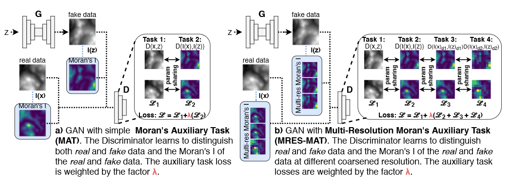
We propose the use of a spatial autocorrelation embedding, the local Moran's I statistic, as an auxiliary learning objective. The local Moran's I measures the direction and extent of each observations correlation to (spatially) neighbouring observations. As such, it serves as a detector of spatial outliers and spatial clusters. We call this approach the Moran's Auxiliary Task (MAT).

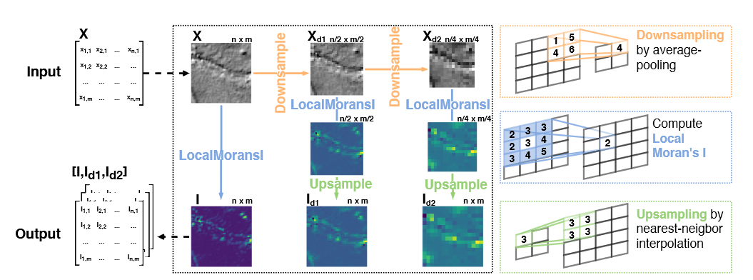
We also propose a novel, multi-resolution local Moran's I statistic to capture spatial dependencies at different spatial scales. This is outlined in the figure above. The multi-resolution local Moran's I can be used for a set of auxiliary tasks; we refer to this approach as Multi-Resolution Moran's Auxiliary Task (MRES-MAT).

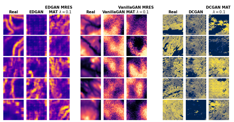
Both approaches can easily be integrated into predictive and generative models; for example GANs, as outlined below. To integrate the auxiliary task(s) into the model loss, we multiply the auxiliary losses by a weight parameter λ. For a more in-depth description of SXL, please see the paper.

SXL in PyTorch

This repository provides a PyTorch implementation of SXL. Let us briefly demonstrate how it works, using a simple example: a CNN conducting a spatial interpolation (regression) task upscaling a 32 x 32 spatial pattern to a 64 x 64 spatial pattern. First, we need to define a multitask CNN:

class CNN_MAT_32(nn.Module):
    """
        CNN w/ Moran's Auxiliary Task
    """
    def __init__(self,  nc=1, ngf=32):
        super(CNN_MAT_32, self).__init__()
        # Shared layers used for data and Moran's I embedding
        self.conv_net = nn.Sequential(nn.ConvTranspose2d(nc,ngf,kernel_size=4,stride=2,padding=1),
          nn.BatchNorm2d(ngf),
          nn.ReLU()
        )
        #Task-specific output layers
        self.output_t1 = nn.Sequential(nn.ConvTranspose2d(ngf,ngf*2,kernel_size=4,stride=2,padding=1),
          nn.BatchNorm2d(ngf*2),
          nn.ReLU(),
          nn.Conv2d(ngf*2,nc,kernel_size=4,stride=2,padding=1),
          nn.Tanh()
        )
        self.output_t2 = nn.Sequential(nn.ConvTranspose2d(ngf,ngf*2,kernel_size=4,stride=2,padding=1),
          nn.BatchNorm2d(ngf*2),
          nn.ReLU(),
          nn.Conv2d(ngf*2,nc,kernel_size=4,stride=2,padding=1),
          nn.Tanh()
        )
    def forward(self, x, y=None):
        mi_x = batch_lw_tensor_local_moran(x.detach().cpu(),w_sparse_32)
        mi_x = mi_x.to(DEVICE)
        y_ = x.view(x.size(0), 1, 32, 32)
        mi_y_ = mi_x.view(mi_x.size(0), 1, 32, 32)
        y_ = self.conv_net(y_)
        mi_y_ = self.conv_net(mi_y_)
        y_ = self.output_t1(y_)
        mi_y_ = self.output_t2(mi_y_)
        return y_, mi_y_

Here, the conv_net module is shared between tasks, i.e. the CNN learns a shared representation of the data AND its local Moran's I embedding. The output layers (output_t1 / output_t2) are task-specific. In the forward() method, we can see the function batch_lw_tensor_local_moran() used to compute the local Moran's I for a whole data batch, taking in a sparse spatial weight matrix w_sparse according to the input size 32 x 32 and the current minibatch x. Our multi-task CNN has two outputs, the predicted 64 x 64 matrix and its predicted local Moran's I embedding.

We can integrate the outputs into a multi-taks loss as follows:

for e in range(num_epochs):
    # Within each iteration, we will go over each minibatch of data
    for minibatch_i, (y_batch,x_batch) in enumerate(train_loader):
      # Get data
      x = x_batch.to(DEVICE)
      y = y_batch.to(DEVICE)
      # Prepare input
      x = x[:,0,:,:].reshape(batch_size,1,32,32)
      # Prepare output
      mi_y = y[:,1,:,:].reshape(batch_size,1,64,64) #Local Moran's I of the output can be precomputed
      y = y[:,0,:,:].reshape(batch_size,1,64,64)
      # Training Net
      x_outputs, mi_x_outputs = CNN(x)
      CNN_x_loss = criterion(x_outputs, y)
      CNN_mi_x_loss = criterion(mi_x_outputs, mi_y)
      CNN_loss = CNN_x_loss + lambda_ * (CNN_mi_x_loss)
      CNN.zero_grad()
      CNN_loss.backward()
      CNN_opt.step()

Here, lamda_ = λ, the auxiliary loss weight parameter. In our experiments, we work with lambda values [0.01, 0.1, 1], however we also provide an Example notebook showing how each tasks uncertainty can be used to weight the losses.

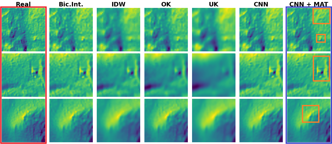
How does it work? Like a charm! Below are some interpolation examples from our CNN MAT, compared to the "Vanilla" CNN and common spatial interpolation benchmarks.

Compute MRES-MAT

To also quickly demonstrate how to compute the multi-resolution local Moran's I, let's assume we have an input of size 32 x 32 and want to compute the Moran's I at the original resolution and downsampled by factor 2 and 4. To do this, we first downsample the input (using average pooling operations), then compute the local Moran's I statistic and upsample again (using nearest neighbor interpolation) to the original 32 x 32 input size. Given an input batch x, the according PyTorch code looks like this:

x_d1 = downsample(x)
x_d2 = downsample(x_d1)
mi_x = batch_lw_tensor_local_moran(x.detach().cpu(),w_sparse_32)
mi_x_d1 = batch_lw_tensor_local_moran(x_d1.detach().cpu(),w_sparse_16)
mi_x_d2 = batch_lw_tensor_local_moran(x_d2.detach().cpu(),w_sparse_8)
mi_x_d1 = nn.functional.interpolate(mi_x_d1,scale_factor=2,mode="nearest")
mi_x_d2 = nn.functional.interpolate(mi_x_d2,scale_factor=4,mode="nearest")

mi_x is the local Moran's I of the original data, mi_x_d1 and mi_x_d2 the coarsened Moran's I (factor 2 and 4).

Examples

We currently provide the following examples for you to test out:

• Example 1: Generative modeling with MAT
• Example 2: Generative modeling with MRES-MAT
• Example 3: Predictive modeling (spatial interpolation) with MAT
• Example 4: Generative modeling with MRES-MAT and uncertainty weights.

Citation

@inproceedings{
    klemmer2021sxl,
    author = {Klemmer, Konstantin and Neill, Daniel B.},
    title = {Auxiliary-Task Learning for Geographic Data with Autoregressive Embeddings},
    year = {2021},
    isbn = {9781450386647},
    publisher = {Association for Computing Machinery},
    address = {New York, NY, USA},
    url = {https://doi.org/10.1145/3474717.3483922},
    doi = {10.1145/3474717.3483922},
    booktitle = {Proceedings of the 29th International Conference on Advances in Geographic Information Systems},
    pages = {141–144},
    numpages = {4},
    location = {Beijing, China},
    series = {SIGSPATIAL '21}
}