- Overview
- Results
- Executable
Peer-review published paper for this technique can be found here:
https://github.com/jose-villegas/VCTRenderer/blob/master/paper_final.pdf http://ieeexplore.ieee.org/abstract/document/7833375/
My thesis can be found here (Spanish) here: https://raw.githubusercontent.com/jose-villegas/ThesisDocument/master/Tesis.pdf
Computing indirect illumination is a challenging and complex problem for real-time rendering in 3D applications. This global illumination approach computes indirect lighting in real time utilizing a simplified version of the outgoing radiance and the scene stored in voxels.
Deferred voxel shading is a four-step real-time global illumination technique inspired by voxel cone tracing and deferred rendering. This approach enables us to obtain an accurate approximation of a plethora of indirect illumination effects including: indirect diffuse, specular reflectance, color-blending, emissive materials, indirect shadows and ambient occlusion. The steps that comprehend this technique are described below.
| Technique Overview |
|---|
 |
The first step is to voxelize the scene, my implemention voxelizes scene albedo, normal and emission to approximate emissive materials. For this conservative voxelization and atomic operations on 3D textures are used as described here.
...
layout(binding = 0, r32ui) uniform volatile coherent uimage3D voxelAlbedo;
layout(binding = 1, r32ui) uniform volatile coherent uimage3D voxelNormal;
layout(binding = 2, r32ui) uniform volatile coherent uimage3D voxelEmission;
...
// average normal per fragments sorrounding the voxel volume
imageAtomicRGBA8Avg(voxelNormal, position, normal);
// average albedo per fragments sorrounding the voxel volume
imageAtomicRGBA8Avg(voxelAlbedo, position, albedo);
// average emission per fragments sorrounding the voxel volume
imageAtomicRGBA8Avg(voxelEmission, position, emissive);
...| Scene | Average Albedo | Average Normal | Average Emission |
|---|---|---|---|
 |
 |
 |
 |
My voxel structure is inspired by deferred rendering, where a G-Buffer contains relevant data to later be used in a separate light pass. Normal, albedo and emission values are stored in voxels during the voxelization process, every attribute has its own 3D texture associated. This information is sufficient to calculate the diffuse reflectance and normal attenuation on a separate light pass where, instead of computing the lighting per pixel it is done per voxel. The structure can be extended to support a more complicated reflectance model but this may imply a higher memory consumption to store additional data.
Furthermore, another structure is used for the voxel cone tracing pass. The resulting values of the lighting computations per voxel are stored in another 3D texture which we will call radiance volume. To approximate the incrementing diameter of the cone, and its sampling volume, levels of detail of the voxelized scene are used. For anisotropic voxels six 3D textures at half resolution of the radiance volume are required, one per every axis direction positive and negative, the levels of details are stored within the mipmap levels of these textures which we will call directional volumes.
The radiance volume represents the maximum level of detail for the voxelized scene, this texture is separated from the directional volumes. To bind these two structures, linear interpolation is used between samples of both structures when the mipmap level required for the diameter of the cone ranges between, the maximum level and the first filtered level of detail.
| A visualization of the voxel structure |
|---|
 |
For dynamic updates, the conservative voxelization of static and dynamic geometry are separated. While static voxelization happens only once, dynamic voxelization happens per frame or when needed. The voxelization for both types of geometry rely on the same process, hence a way to indicate which voxels are static is needed. In my approach I use a single value 3D texture to identify voxels as static, this texture will be called flag volume.
During static voxelization, after a voxel is generated a value is written to the flag volume indicating this position as static. In contrast, during the dynamic voxelization, before generating a voxel, a value is read from the flag volume at the writing position of the voxel, if the value indicates this position is marked as static then writing is discarded, leaving the static voxels untouched.
To constantly revoxelize the scene it is necessary to clear from the 3D textures the previous stored dynamic voxels. This is done before the dynamic voxelization using compute shaders. The flag volume is read to clear voxels under two conditions: if the voxel exists and if it’s dynamic.
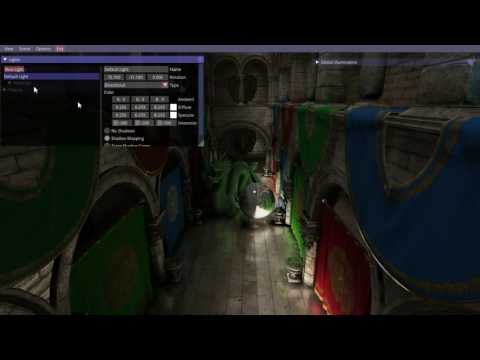
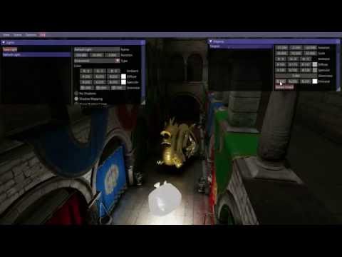
The second step is voxel illumination, for this we calculate the outgoing radiance per voxel using the data stored from the voxelization step. For this we only need the voxel normal, and its position which can be easily extracted by projecting the voxel 3D coordinates in world-space, then we can calculate the direct lighting per voxel. This is all done in a compute shader.
One of the advantages of this technique is that it's compatible with all standard light types like point, spot and directional lights, another is that we don't need shadow maps, though they can help greatly with precision specially for directional lights. Other techniques calculate the voxel radiance per light's shadow map, meaning that for every shadow-mapped light that wants to contribute to the voxel radiance the illumination step has to be repeated.
| Scene | Voxel Direct Lighting |
|---|---|
|
 |
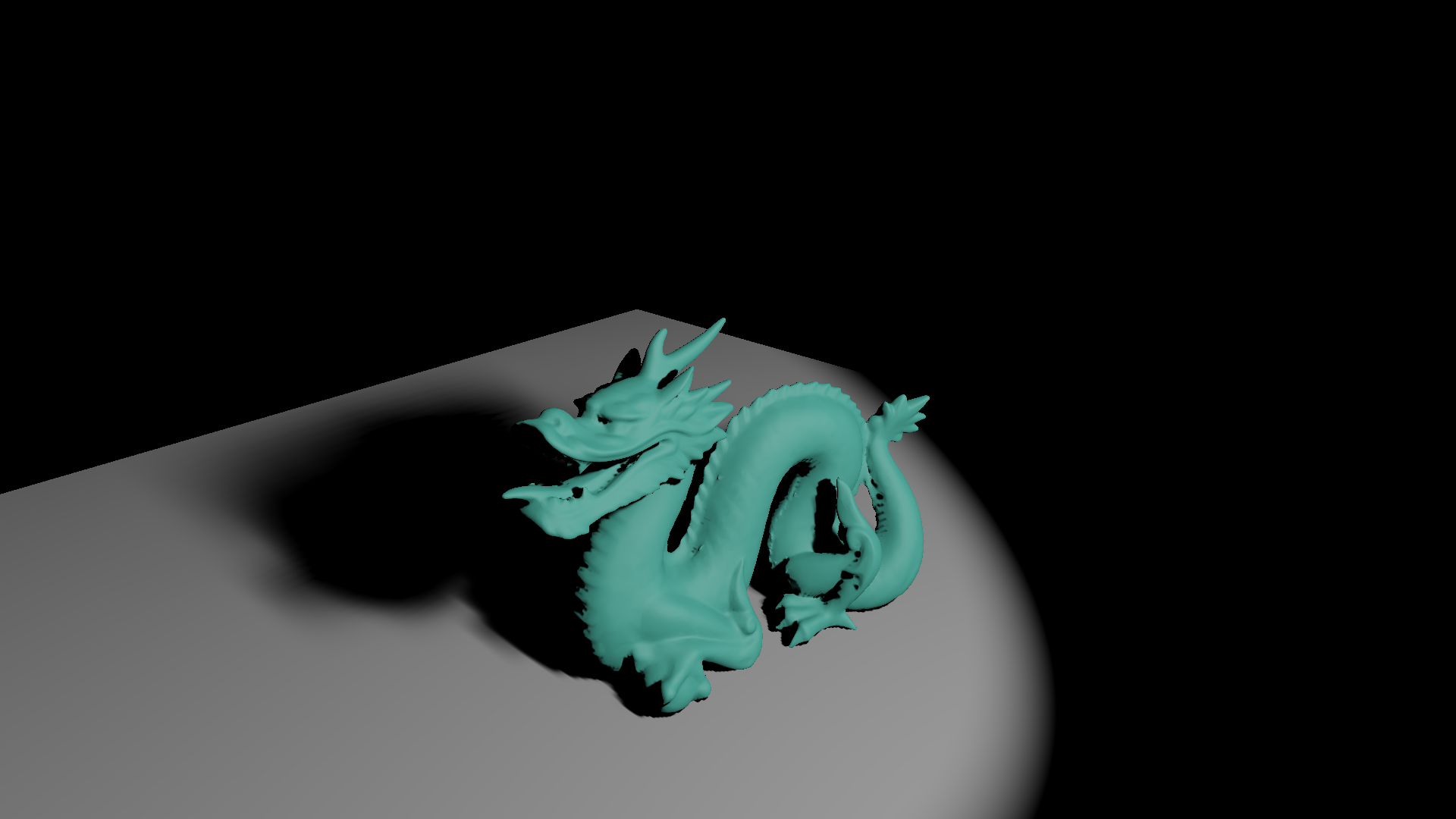
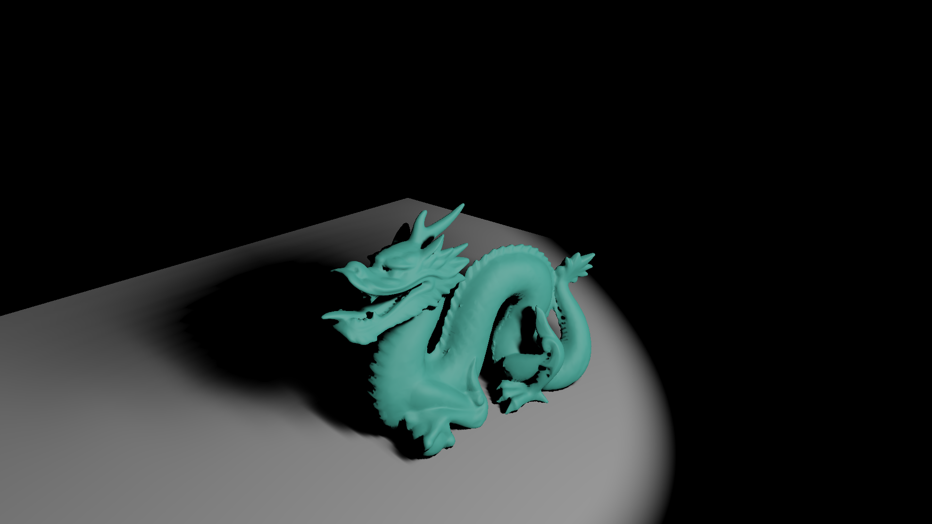
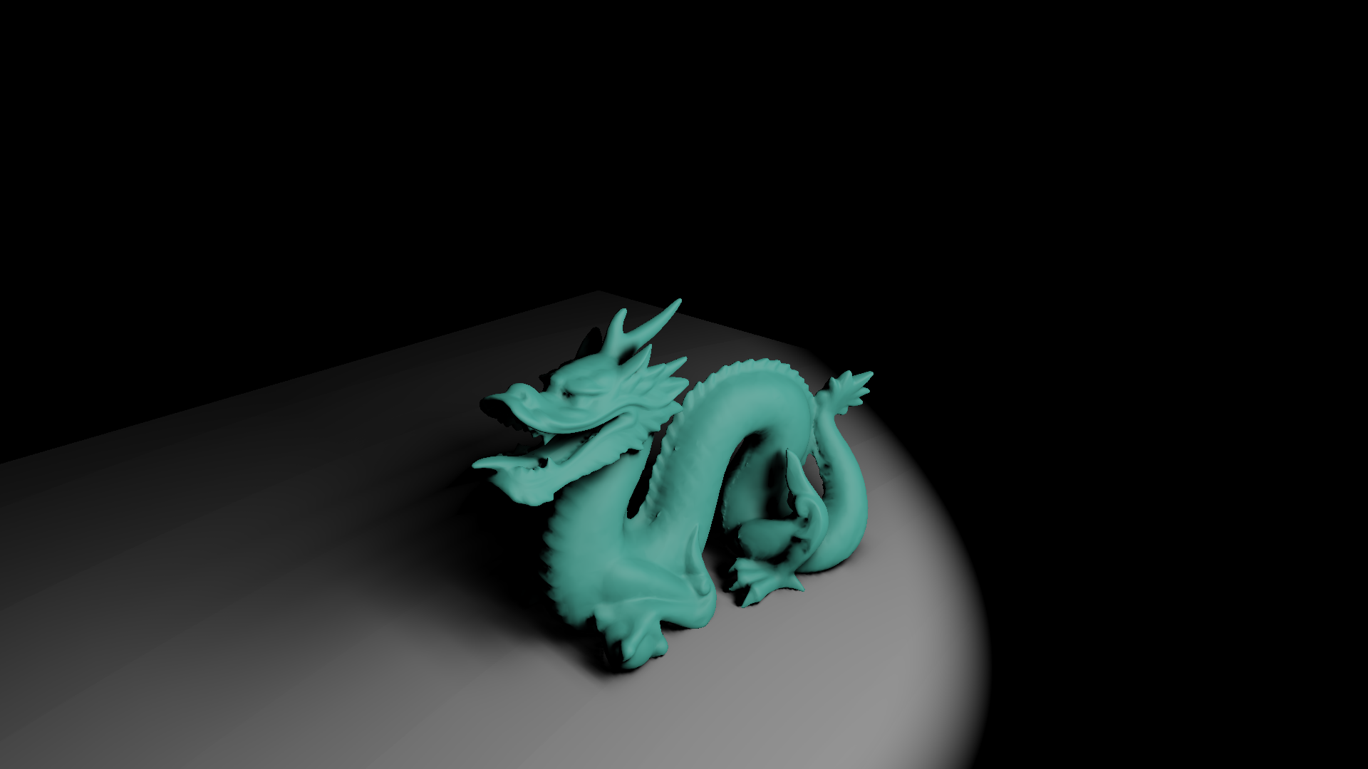
A disvantage of this technique is the loss of precision averaging all the geometry normals within a voxel. The resulting averaged normal may end up pointing towards a non-convenient direction. This problem is notable when the normal vectors within the space of a voxel are uneven:

To reduce this issue my proposal utilizes a normal-weighted attenuation, where first the normal attenuation is calculated per every face of the voxel as follows:
Then three dominant faces are selected depending on the axes sign of the voxel averaged normal vector:
And finally, the resulting attenuation is the product of every dominant face normal attenuation, multiplied with the weight per axis of the averaged normal vector of the voxel, the resulting reflectance model is computed as follows:
where is the light source intensity,
the voxel albedo,
the normal vector of the voxel and
the light direction.
| Normal Attenuation | Normal-weighted Attenuation |
|---|---|
 |
 |
To generate accurate results during the cone tracing step the voxels need to be occluded, otherwise voxelized geometry that is supposed to have little to no outgoing radiance will contribute to the indirect lighting calculations.
The classic shadow mapping or alike techniques can be used to compute the voxels occlusion. The position of the voxel is projected in light space and the depth of the projected point is compared with the stored depth from the shadow map to determine if the voxel is occluded.
My proposal also computes occlusion using raycasting within a volume. Any of the resulting volumes from the voxelization process can be used since the algorithm only needs to determine if a voxel exists at a certain position. To determine occlusion of a voxel, a ray is traced from the position of voxel in the direction of the light, the volume is sampled to determine if at the position of the ray there is a voxel, if this condition is true then the voxel is occluded.
Instead of stopping the ray as soon a voxel is found, soft shadows can be approximated with a single ray accumulating a value \ per collision and dividing by the traced distance
, i.e.
, where
represents the occlusion value after the accumulation is finished. This technique exploits the observation that, from the light point of view, the number of collisions will usually be higher for the rays that pass through the borders of the voxelized geometry.
| Hard Voxel Shadows | Soft Voxel Shadows |
|---|---|
 |
 |
 |
 |
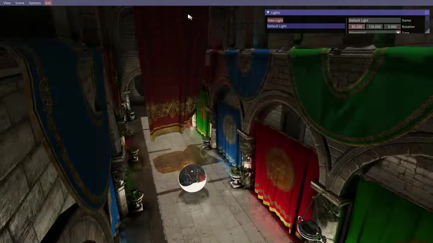
Adding to the final radiance value the emission term can be used approximate emissive surfaces such as area lights, neon lights, digital screens, etc., this provides a crude approximation of the emission term the rendering equation. After the direct illumination value is obtained the emission term from the voxelization process is added to this value per voxel. During the cone tracing step, these voxels will appear to be bright even on occluded areas, hence indirect light is accumulated per cone from these regions of the voxelized scene.
For more precise results during the cone tracing step anisotropic voxels are used. The mipmapping levels, as seen in the directional volumes in the voxel structure, will store per every voxel six directional values, one per every directional axis positive and negative. Each cone has an origin, aperture angle and direction, this last factor determines which three volumes are sampled. The directional sample is obtained by linearly interpolating the three samples obtained from the selected directional volumes.
To generate the anisotropic voxels I use the process detailed by Crassin here. To compute a directional value a step of volumetric integration is done in depth and the directional values are averaged to obtain the resulting value for a certain direction. In my approach this is done using compute shaders, executing a thread per every voxel at the mipmap level that is going to be filtered using the values from the previous level, this process is done per every mipmap level.
| Process to generate anisotropic voxels |
|---|
 |
Voxel cone tracing is similar to ray marching, the cone advances a certain length every step, except that the sampling volume increases along the diameter of the cone. The mipmap levels in the directional volumes are used to approximate the expansion of the sampling volume during the cone trace, to ensure smooth variation between samples quadrilinear interpolation is used which is natively supported with graphics hardware for 3D textures. This step is done in the fragment shader as a screenspace effect, a deferred rendering backend is needed, though voxel cone tracing can be done in forward rendering regardless, it would be extremely inneficient and expensive.
The shape of the cone is meant to exploit the spatial and directional coherence of the many rays packed within the space of a cone. This behavior is used in many approaches such as packet ray-tracing.
| Visual representation of a cone used for cone tracing |
|---|
 |
As seen in the figure above each cone is defined by an origin , a direction
and an aperture angle
. During the cone steps the diameter of the cone is defined by
, this value can be extracted using the traced distance
with the following equation:
. Which mipmap level should be sampled depending on the diameter of the cone can be obtained using the following equation:
, where
is the size of a voxel at the maximum level of detail.
As described by Crassin here, for each cone trace we keep track of the occlusion value and the color value
which represents the indirect light towards the cone origin
. In each step we retrieve from the voxel structure the occlusion value
and the outgoing radiance
. Then the
and
values are updated using volumetric front-to-back accumulation as follows:
and
.
To ensure good integration quality between samples the distance between steps is modified by a factor
. With
the value of
is equivalent to the current diameter
of the cone, values less than 1 produce higher quality results but require more samples which reduces the performance.
Indirect lighting is approximated with a crude Monte Carlo approximation. The hemisphere region for the integral in the rendering equation can be partitioned into a sum of integrals. For a regular partition, each partitioned region resembles a cone. For each cone their contribution is approximated using voxel cone tracing, the resulting values are then weighted to obtain the accumulated contribution at the cones origin.
The distribution of the cones matches the shape of the BRDF, for a Blinn-Phong material a few large cones distributed over the normal oriented hemisphere estimate the diffuse reflection, while a single cone in the reflected direction, where its aperture depends on the specular exponent, approximates the specular reflection.
| Diffuse Cones | Specular Cone | BRDF |
|---|---|---|
 |
 |
 |
Ambient occlusion can be approximated using the same cones used for the diffuse reflection for efficiency. For the ambient occlusion term we only accumulate the occlusion value
, at each step the accumulated value is multiplied with the weighting function
, where
is the current radius of the cone and
an user defined value which controls how fast
decays along the traced distance. At each cone step the ambient occlusion term is updated as:
.
Cone tracing can also be used to achieve soft shadows tracing a cone from the surface point x towards the direction of the light The cone aperture controls how soft and scattered the resulting shadow is. For soft shadows with cones we only accumulate the occlusion value at each step.
| Cone Soft Shadows |
|---|
 |
To calculate the diffuse reflection over a surface point using voxel cone tracing we need its normal vector, albedo and the incoming radiance at that point. Since we voxelize the geometry normal vectors and the albedo into 3D textures, all the needed information for the indirect diffuse term is available after calculating the voxel direct illumination. In my approach I perform voxel cone tracing per voxel using compute shaders to calculate the first bounce of indirect diffuse at each voxel. This step is done after the outgoing radiance values from the voxel direct illumination pass are anisotropically filtered.
For each voxel we use its averaged normal vector to generate a set of cones around the normal oriented hemisphere to calculate the indirect diffuse at the position of the voxel. The weighted result from all the cones is then multiplied by the albedo of the voxel and added to the direct illumination value. The resulting outgoing radiance for the radiance volume now stores the direct illumination, and the first bounce of indirect diffuse. The anisotropic filtering process needs be repeated for the new values. This enables us to approximate the second bounce of indirect lighting during the final voxel cone tracing step per pixel. This can be extended to support multiple bounces.
The results here were tested on an AMD 380 R9 GPU on different scenes with increasing geometric complexity and dynamic objects added to the scene. The scenes used for testing are listed below:
| Name | Model | Vertices | Triangles |
|---|---|---|---|
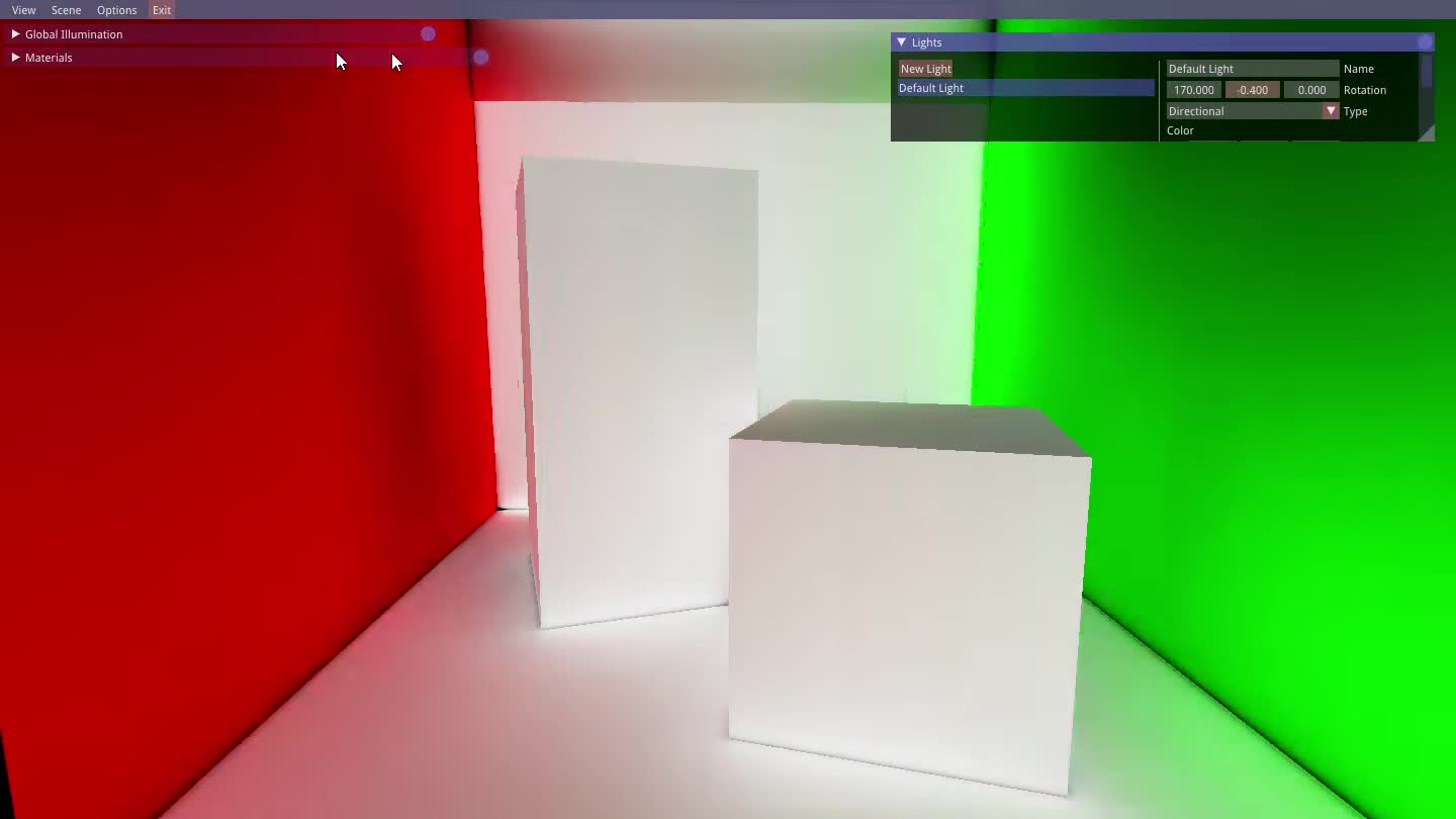
| S1 | Cornell Box | 72 | 36 |
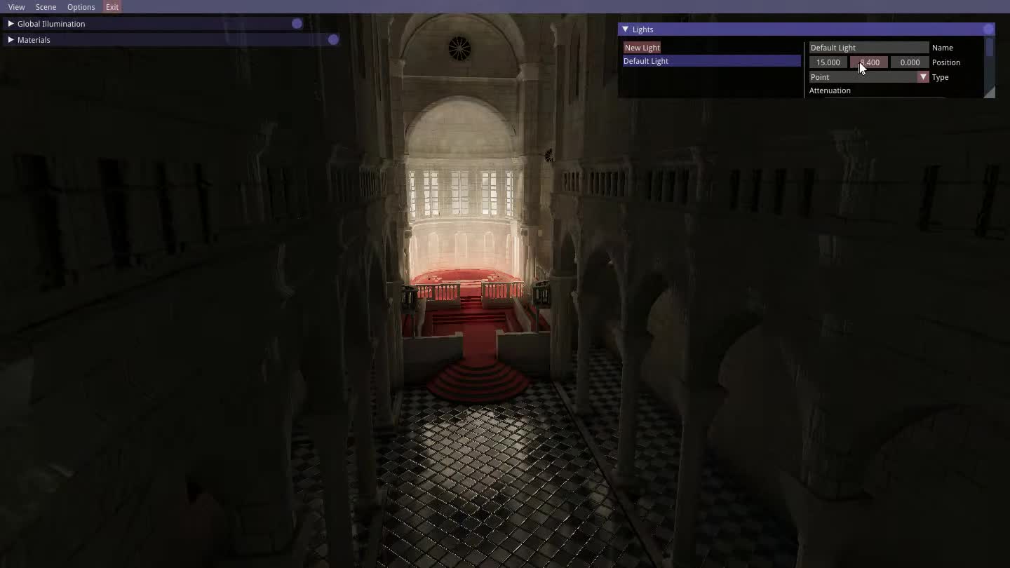
| S2 | Sibenik Cathedral | 40.479 | 75.283 |
| S3 | Crytek Sponza | 153.635 | 278.163 |
The times per frame for the dynamic and static voxelization of each scene are show below:
| Name | Static | Clear Dynamic | Dynamic |
|---|---|---|---|
| S1 | 0.51 ms | 0.78 ms | 1.30 ms |
| S2 | 1.80 ms | 0.58 ms | 2.11 ms |
| S3 | 11.29 ms | 0.60 ms | 2.03 ms |
For the voxelization process, a higher resolution for the voxel representation can actually be beneficial, because it reduces thread collisions for the writing operations, in the scene S3 there is a higher time for the static voxelization this reason, S3 has a higher triangle density per voxel meaning more syncing operations are needed.
The table below shows the results for voxel direct illumination with shadow mapping or raycasting for voxel occlusion and voxel global illumination, it also includes the time for anisotropic filtering after both steps. For voxel direct illumination the times are similar between all scenes using shadow mapping, while raycasting costs more performance it enables occlusion for any type of light source without shadow mapping.
| Name | Direct (with Shadow Mapping) | Direct (with Raycasting) | Anistropic Filtering | Global Illumination | Anistropic Filtering |
|---|---|---|---|---|---|
| S1 | 1.33 ms | 20.32 ms | 1.39 ms | 8.41 ms | 1.38 ms |
| S2 | 0.95 ms | 4.57 ms | 1.38 ms | 3.88 ms | 1.37 ms |
| S3 | 1.13 ms | 3.31 ms | 1.37 ms | 5.44 ms | 1.38 ms |
For raycasting, the amount of empty space in the scene affects how early the traced rays end, which affects the general performance. For high density scenes such as S3 most rays end early, in contrast the scene S1 takes a considerable amount of time using raycasting because the scene is mostly empty space, this same condition also applies for the voxel indirect diffuse step.
| Scene | Voxel Direct | Voxel Direct + Indirect Diffuse |
|---|---|---|
 |
 |
 |
 |
 |
 |
 |
 |
 |
Once the voxel structure is anisotropically filtered we can proceed with voxel cone tracing per pixel for the final composition of the image. In my approach six cones with an aperture of 60 degrees are used to approximate the indirect diffuse term, for the indirect specular in these test I utilize a specular cone with an aperture of 10 degrees. The next table shows the performance for indirect lighting on different scenes. For all the scenes my implementation achieves results over 30FPS ( < 33.3 ms ) under constant dynamic update, meaning objects and lights are changing and moving per frame. The dynamic update includes dynamic voxelization, voxel direct illumination, voxel global illumination and the necessary anistropic filtering steps. For a screen resolution of 1920x1080 pixels my implementation obtains an average framerate of 28.57 ms for the scene S3, 27.02 ms for S2 and 27.77 ms for S1 under constant dynamic update, these results show that even with a high resolution the technique can achieve over 30FPS for all the scenes.
| Scene | Direct | Indirect (Diffuse + Specular) | Direct + Indirect | Dynamic Stress |
|---|---|---|---|---|
| S1 | 1.03 ms | 7.27 ms | 7.67 ms | 17.81 ms |
| S2 | 1.32 ms | 7.62 ms | 8.32 ms | 17.60 ms |
| S3 | 1.34 ms | 7.81 ms | 8.41 ms | 16.97 ms |
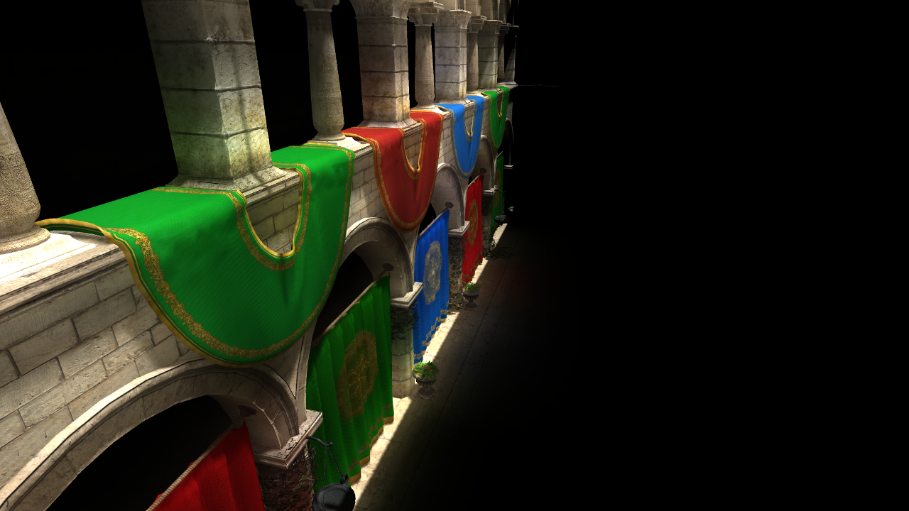
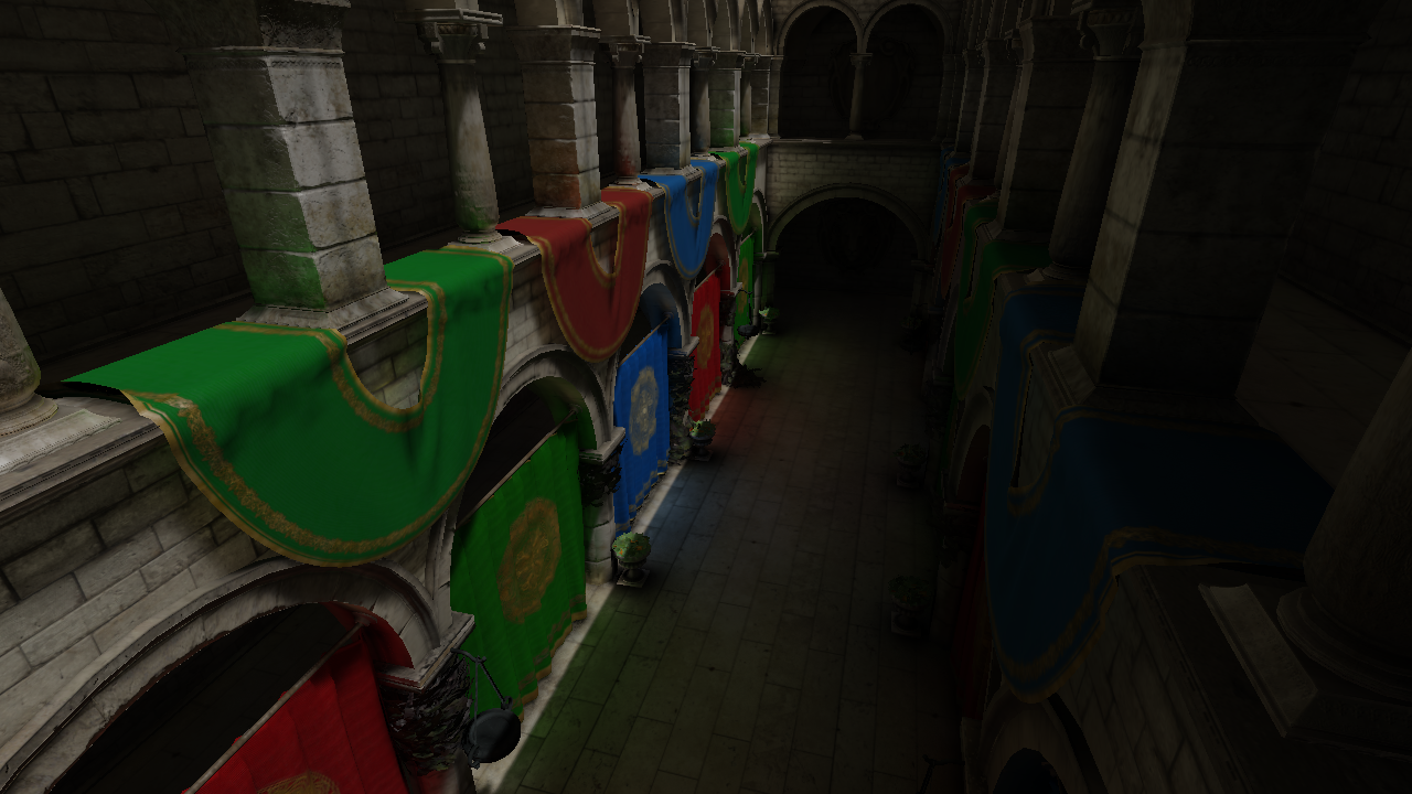
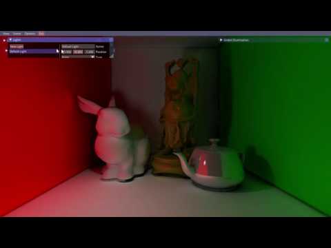
Below a visual comparison between a reference image rendered in a path-tracer for 3 hours, another real time global illumination technique called light propagation volumes and my technique. The image generated by my technique is closer to the reference image, specially the indirect diffuse reaching the right columns that aren't directly hit by the light source. Light propagation volumes is also limited in the sense that it only provides approximation for the indirect diffuse term, whereas voxel cone tracing achieves specular reflection and many other light phenomena.
| Reference (3~ hours) | Light Propagation Volumes (18.86 ms) | My approach (17.34 ms) |
|---|---|---|
 |
 |
 |
In my implementation the dynamic update can be set to update at a given number of frames or on demand, a simple optimization for example is to update each 5~3 frames, this can easily give results over 60FPS for most scenes with little to zero notable difference.
Since the lighting step is separate from the voxelization step, revoxelization is only truly needed when objects move within the scene. For changes that only involve lighting revoxelization is unnecesary.
One optimization to consider that wasn't implemented in my application is to separate the indirect lighting calculation from voxel cone tracing at a lower resolution. The higher the resolution the more surface points that need to be cone traced since each pixel represents a position in scene. A disvantage of doing this is that it creates some notable artifacts, though they can be somewhat reduced through clever use of screen-space techniques.
| Cornell Box | Sibenik Cathedral | Crytek Sponza |
|---|---|---|
 |
 |
 |
(These are videos)
| Emissive Material | Indirect Shadows |
|---|---|
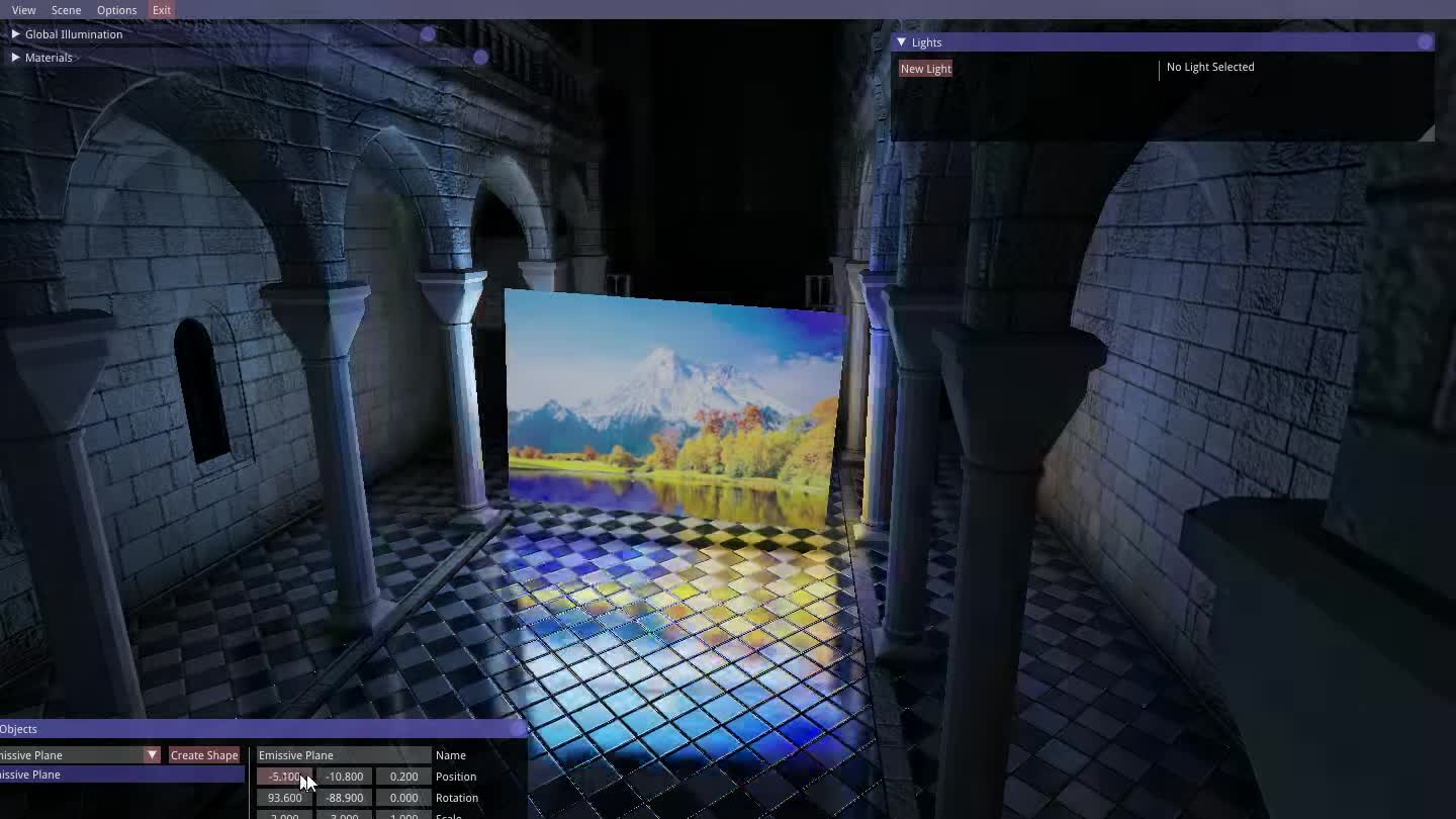 |
 |
(These are videos)
| Cornell Box | Sibenik Cathedral | Crytek Sponza |
|---|---|---|
 |
 |
 |
| 1 degree aperture | 5 degree aperture | 10 degree aperture | 25 degree aperture |
|---|---|---|---|
 |
 |
 |
 |
 |
 |
 |
 |
 |
 |
 |
 |
The executable application for this technique can be found in this link here Press Shift + F to enable free camera mode.