R package BridgeChange constains functions useful to analyze
time-series data and panel data with possibly large number of covariates
and change-points. This package offers a Bayesian inference on the
linear regression mode under high-dimensinal covariates whose effects on
the outcome are allowed to be heterogeneous across time. This package
will be useful to discover a set of predictive variables under dynamic
setting where time-varying effect is expected to exist in many cases.
You can install the most recent version of BridgeChange from Gitub
using the devtools package.
# install BridgeChange from Github
# you might need to instal "devtools"
devtools::install_github("jongheepark/BridgeChange")
#> Downloading GitHub repo jongheepark/BridgeChange@HEAD
#> collapse (1.7.5 -> 1.7.6) [CRAN]
#> Installing 1 packages: collapse
#> Installing package into '/Users/park/.R/packages'
#> (as 'lib' is unspecified)
#>
#>   There is a binary version available but the source version is later:
#>          binary source needs_compilation
#> collapse  1.7.5  1.7.6              TRUE
#> installing the source package 'collapse'
#> Warning in i.p(...): installation of package 'collapse' had non-zero exit status
#>      checking for file ‘/private/var/folders/tf/xj58_m8146s8_tsg2989y7p80000gn/T/RtmpXSStBH/remotes543210316b5c/jongheepark-BridgeChange-fbc7a23/DESCRIPTION’ ...  ✓  checking for file ‘/private/var/folders/tf/xj58_m8146s8_tsg2989y7p80000gn/T/RtmpXSStBH/remotes543210316b5c/jongheepark-BridgeChange-fbc7a23/DESCRIPTION’
#>   ─  preparing ‘BridgeChange’:
#>      checking DESCRIPTION meta-information ...  ✓  checking DESCRIPTION meta-information
#>   ─  cleaning src
#>   ─  checking for LF line-endings in source and make files and shell scripts
#>   ─  checking for empty or unneeded directories
#>   ─  building ‘BridgeChange_1.4.tar.gz’
#>
#>
#> Installing package into '/Users/park/.R/packages'
#> (as 'lib' is unspecified)The following two model arguments are availabel for the fixed-effects
HMBB. - the fixed effects model ("within"), the default, - the pooling
model ("pooling"),
We will use the one-way (time) fixed effect model because the original model has a time-invariant covariate (central).
model = "within"
index = c('country', 'year')
effect = 'time'
formula <- growth ~ lagg1 + opengdp + openex + openimp + leftc * central
pdata   <- pdata.frame(data, index)
pm <- plm(formula, data = pdata, model = model, effect = effect)
summary(pm)
#> Oneway (time) effect Within Model
#>
#> Call:
#> plm(formula = formula, data = pdata, effect = effect, model = model)
#>
#> Balanced Panel: n = 16, T = 15, N = 240
#>
#> Residuals:
#>      Min.   1st Qu.    Median   3rd Qu.      Max.
#> -5.837357 -1.197473  0.067401  1.170477  4.529090
#>
#> Coefficients:
#>                  Estimate  Std. Error t-value  Pr(>|t|)
#> lagg1          0.05031487  0.13920445  0.3614 0.7181162
#> opengdp       -0.00233019  0.00186733 -1.2479 0.2134164
#> openex         0.00200753  0.00120757  1.6625 0.0978586 .
#> openimp       -0.00060892  0.00167894 -0.3627 0.7171955
#> leftc         -0.02471232  0.00927578 -2.6642 0.0082944 **
#> central       -0.76356330  0.21625824 -3.5308 0.0005055 ***
#> leftc:central  0.01286831  0.00361409  3.5606 0.0004542 ***
#> ---
#> Signif. codes:  0 '***' 0.001 '**' 0.01 '*' 0.05 '.' 0.1 ' ' 1
#>
#> Total Sum of Squares:    809.01
#> Residual Sum of Squares: 718.43
#> R-Squared:      0.11196
#> Adj. R-Squared: 0.026415
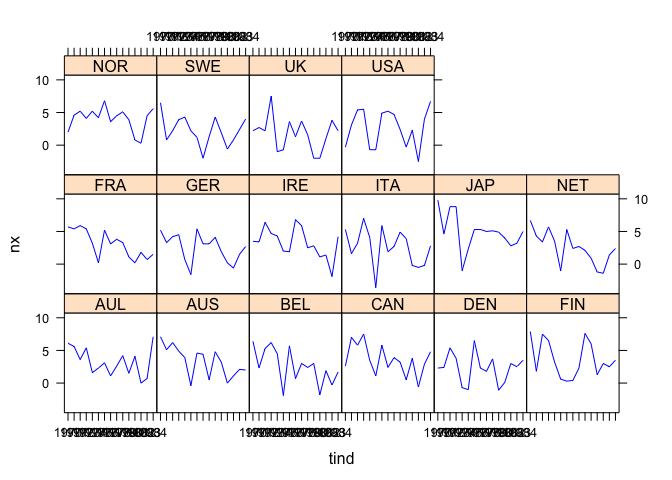
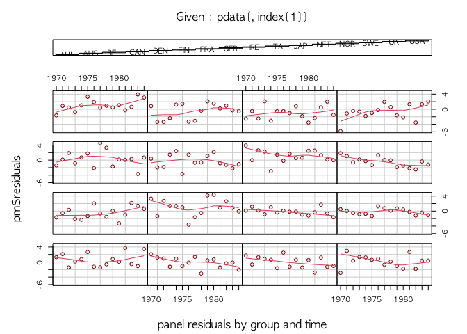
#> F-statistic: 3.92636 on 7 and 218 DF, p-value: 0.00046809We take a look at the response data and panel residuals to check the sign of misfit due to time-varying effects.
## response
plot(pdata$growth)## panel residuals
coplot(pm$residuals ~ pdata[,index[2]]|pdata[,index[1]], data=pdata, ## number=length(unique(pdata[,index[1]])),
overlap=.1, col="brown", type="l",
panel = panel.smooth, xlab="panel residuals by group and time")We fit three HMBBs with no break, one break, and two breaks to see
whether effects of covariates change over time. To save time, we set
mcmc = 100 here. BridgeFixedPanel transforms the panel data using
plm arguments of model, effect and index first. Then, it fits
HMBB on the transformed data. n.break sets the number of break to be
estimated.
mcmc = 100; burn = 100; verbose = 100; thin = 1;
formula <- growth ~ lagg1 + opengdp + openex + openimp + leftc + central + inter
agl.cp0 <- BridgeFixedPanel(formula=formula, data = data,
                            model = model, index = index, effect = effect,
                            mcmc=mcmc, verbose=verbose, Waic = TRUE,
                            n.break = 0)
#> Initializing betas by SLOG
#> ----------------------------------------------------
#> MCMC SparseChangeMixedPanel Sampler Starts!
#> Initial state =  15
#> ----------------------------------------------------
#>
#> ----------------------------------------------
#> ## iteration =  100
#> ----------------------------------------------
#> beta:   0.0019 -0.2741  0.0991  0.1055 -0.4680 -0.1523  0.6372
#>
#> ----------------------------------------------
#> ## iteration =  200
#> ----------------------------------------------
#> beta:   0.054 -0.146  0.638 -0.304 -0.480 -0.395  0.740
#>
#> ----------------------------------------------
#>  Likelihood computation
#>     loglike:  -326.3751
#> ----------------------------------------------
#>
#> ----------------------------------------------
#>  Waic:  668.6554
#>  run time:  0.826
#> ----------------------------------------------
agl.cp1 <- BridgeFixedPanel(formula=formula, data = data,
                            model = model, index = index, effect = effect,
                            mcmc=mcmc, verbose=verbose, Waic = TRUE,
                            n.break = 1)
#> Initializing betas by SLOG
#> ----------------------------------------------------
#> MCMC SparseChangeMixedPanel Sampler Starts!
#> Initial state =  9 6
#> ----------------------------------------------------
#>
#> ----------------------------------------------
#> ## iteration =  100
#> ----------------------------------------------
#> sampled states:  9 6
#> beta at state  1 :  -0.131 -0.070  0.466  0.038 -0.231 -0.863  0.746
#> beta at state  2 :   0.33 -0.14 -0.55  0.47 -0.17  0.38 -0.10
#>
#> ----------------------------------------------
#> ## iteration =  200
#> ----------------------------------------------
#> sampled states:  9 6
#> beta at state  1 :  -0.157 -0.315  0.047  0.739 -0.689 -0.883  1.278
#> beta at state  2 :   0.34 -0.11 -0.63  0.34  0.20  0.32 -0.31
#>
#> ----------------------------------------------
#>  Likelihood computation
#>     loglike:  -308.8235
#> ----------------------------------------------
#>
#> ----------------------------------------------
#>  Waic:  644.8722
#>  run time:  1.703
#> ----------------------------------------------
agl.cp2 <- BridgeFixedPanel(formula=formula, data = data,
                            model = model, index = index, effect = effect,
                            mcmc=mcmc, verbose=verbose, Waic = TRUE,
                            n.break = 2)
#> Initializing betas by SLOG
#> ----------------------------------------------------
#> MCMC SparseChangeMixedPanel Sampler Starts!
#> Initial state =  5 5 5
#> ----------------------------------------------------
#>
#> ----------------------------------------------
#> ## iteration =  100
#> ----------------------------------------------
#> sampled states:  1 8 6
#> beta at state  1 :   0.803 -0.091 -0.469  0.039 -0.146  0.324 -0.242
#> beta at state  2 :  -0.054 -0.155  0.173  0.444 -0.727 -1.020  1.384
#> beta at state  3 :   0.198 -0.417  0.513 -0.449 -0.176  0.143  0.052
#>
#> ----------------------------------------------
#> ## iteration =  200
#> ----------------------------------------------
#> sampled states:  1 8 6
#> beta at state  1 :   0.120  0.212  0.857  0.316  0.293 -0.445  0.035
#> beta at state  2 :  -0.093 -0.006  0.297  0.239 -0.598 -0.894  1.154
#> beta at state  3 :   0.2156 -0.0015  0.3987 -0.4935 -0.1998  0.0900  0.1940
#>
#> ----------------------------------------------
#>  Likelihood computation
#>     loglike:  -303.582
#> ----------------------------------------------
#>
#> ----------------------------------------------
#>  Waic:  643.1039
#>  run time:  2.42
#> ----------------------------------------------
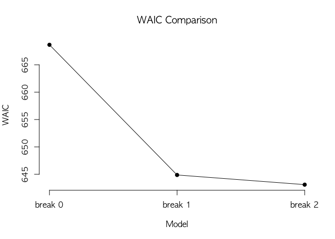
After fitting multiple models, we can compare their model-fits using
WAIC. WaicCompare shows WAIC scores for a list of models. plotWaic()
draws a plot of WAIC scores.
## model selection by WAIC
waic <- WaicCompare(list(agl.cp0, agl.cp1, agl.cp2), print = TRUE)
#>
#> Selected model = break 2
#>
#> [1] 668.66 644.87 643.10
plotWaic(waic)
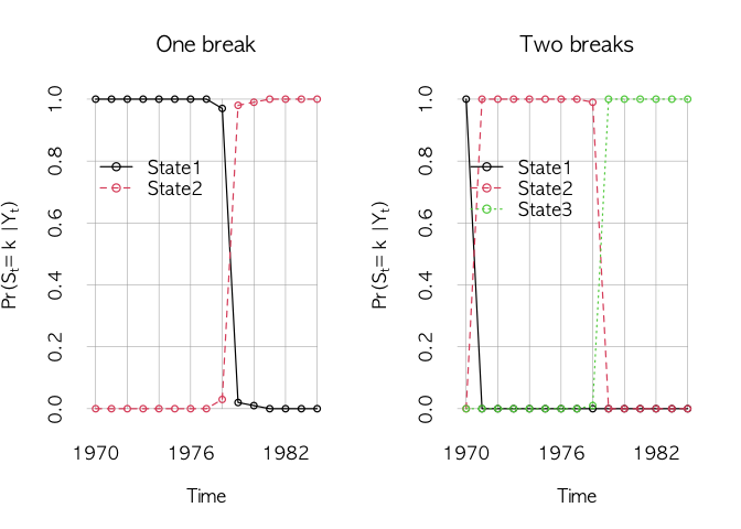
In addition to WAIC, we compare transitions of hidden states.
plotState in MCMCpack can be used to draw hidden state transitions.
## state changes
par(mfrow=c(1, 2))
plotState(agl.cp1, start=1970, legend.control =c(1970, 0.85), main="One break")
plotState(agl.cp2, start=1970, legend.control =c(1970, 0.85), main="Two breaks")
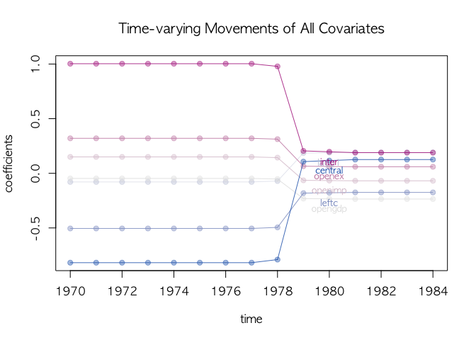
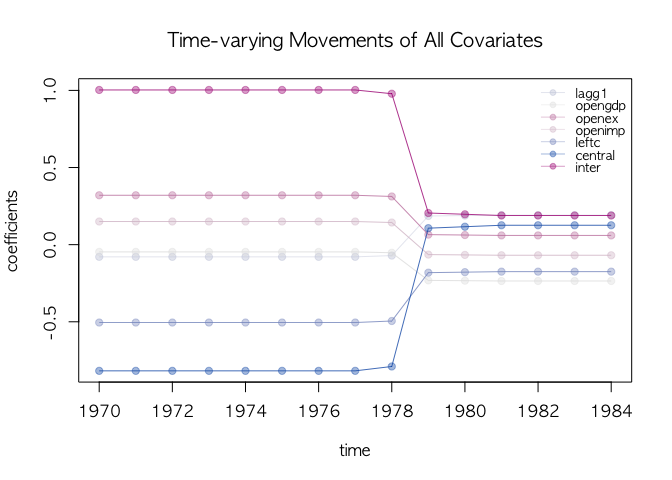
The one break model looks good. We check the time-varying movements of
the one break model using dotplotRegime(). Colors in dotplotRegime()
are determined by the size of coefficients in the first regime. Red
means positive, blue means negative, and grey means close to 0 in the
first regime.
## all covariates
dotplotRegime(agl.cp1, hybrid=FALSE, start = 1970, location.bar=12, x.location="default",
text.cex=0.8, main="Time-varying Movements of All Covariates")## label as a legend
dotplotRegime(agl.cp1, hybrid=FALSE, start = 1970, location.bar=12, x.location="legend",
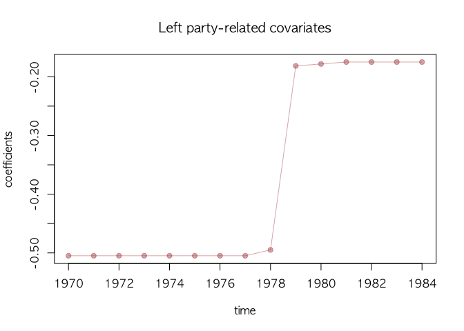
text.cex=0.8, main="Time-varying Movements of All Covariates")We visualize the movement of the selected covariate using select
argument in dotplotRegime(). Here we choose the left-party
government-related variable.
## leftc only
## select works like grep()
dotplotRegime(agl.cp1, hybrid=FALSE, start = 1970, location.bar=12, x.location="static",
              text.cex=0.8, select="left", main=("Left party-related covariates"))