A library for fitting functions to sets of data.
This example illustrates the use of cubic spline interpolation using both natural and forced boundary conditions. Notice, the forced boundary conditions are arbitrarily chosen to illustrate their use.
program example
    use curvefit_core
    use curvefit_interp
    implicit none

    ! Local Variables
    integer(i32), parameter :: knotpts = 9
    integer(i32), parameter :: npts = 1000
    integer(i32) :: i, id
    real(dp) :: dx, dstart, dend, x(knotpts), y(knotpts), xi(npts), y1(npts), &
        y2(npts), xmin, xmax
    type(spline_interp) :: interp

    ! Define a data set:
    x = [-4.0d0, -3.0d0, -2.0d0, -1.0d0, 0.0d0, 1.0d0, 2.0d0, 3.0d0, 4.0d0]
    y = [0.0d0, 0.15d0, 1.12d0, 2.36d0, 2.36d0, 1.46d0, 0.49d0, 0.06d0, 0.0d0]

    ! Interpolate
    xmin = minval(x)
    xmax = maxval(x)
    dx = (xmax - xmin) / (npts - 1.0d0)
    xi(1) = xmin
    do i = 2, npts
        xi(i) = xi(i-1) + dx
    end do

    ! Allow for natural boundary conditions to the spline
    call interp%initialize(x, y)
    y1 = interp%interpolate(xi)

    ! Define the value of the first derivative at the end points
    dstart = 5.0d0
    dend = 0.0d0
    call interp%initialize_spline(x, y, &
        SPLINE_KNOWN_FIRST_DERIVATIVE, dstart, &
        SPLINE_KNOWN_FIRST_DERIVATIVE, dend)
    y2 = interp%interpolate(xi)

    ! Write the results to file
    open(newunit = id, file = "curvefit_interp.txt", action = "write", &
        status = "replace")
    do i = 1, max(knotpts, npts)
        if (i <= knotpts) then
            write(id, '(F14.10AF14.10AF14.10AF14.10AF14.10)') x(i), ",", &
                y(i), ",", xi(i), ",", y1(i), ",", y2(i)
        else
            write(id, '(AF14.10AF14.10AF14.10)') ",,", xi(i), ",", y1(i), &
                ",", y2(i)
        end if
    end do
    close(id)
end program
The above program yields the following data.

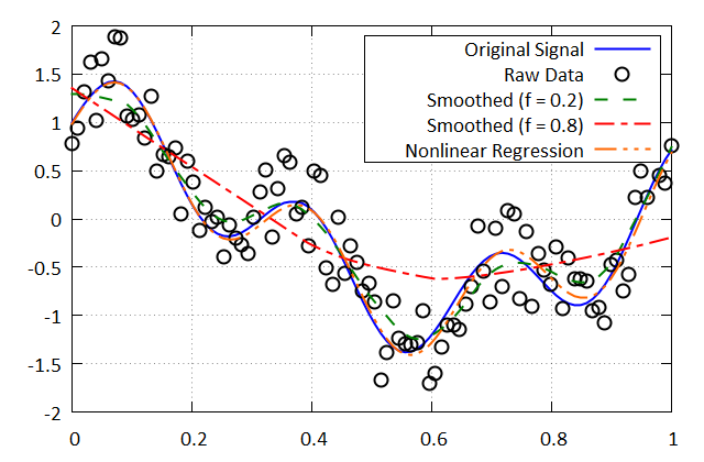
The following example illustrates the use of a robust locally weighted scatterplot smoothing (LOWESS) algorithm to smooth a noisy set of data. The data was generated by adding random values to a known function.
program example
    use curvefit_core
    use curvefit_regression
    implicit none

    ! Parameters
    integer(i32), parameter :: n = 100
    real(dp), parameter :: maxX = 1.0d0
    real(dp), parameter :: minX = 0.0d0

    ! Local Variables
    integer(i32) :: i, id
    real(dp) :: x(n), y(n), yr(n), ys(n), ys2(n), dx, cnl(5), ynl(n)
    type(lowess_smoothing) :: fit
    type(nonlinear_regression) :: solver
    procedure(reg_fcn), pointer :: fcn

    ! Initialization
    dx = (maxX - minX) / (n - 1.0d0)
    x(1) = minX
    do i = 2, n
        x(i) = x(i-1) + dx
    end do
    y = 0.5d0 * sin(2.0d1 * x) + cos(5.0d0 * x) * exp(-0.1d0 * x)
    call random_number(yr)
    yr = y + (yr - 0.5d0)

    ! Generate the fit
    call fit%initialize(x, yr)
    ys = fit%smooth(0.2d0)
    ys2 = fit%smooth(0.8d0)

    ! For comparison purposes, consider a nonlinear regression fit.  As we know
    ! the coefficients, they provide a very good starting guess.
    cnl = [0.5d0, 2.0d0, 20.0d0, 5.0d0, -0.1d0]
    fcn => nrfun
    call solver%initialize(x, yr, fcn, size(cnl))
    call solver%solve(cnl)
    do i = 1, n
        ynl(i) = fcn(x(i), cnl)
    end do

    ! Display the computed coefficients
    print '(A)', "f(x) = c0 * sin(c1 * x) + c2 * cos(c3 * x) * exp(c4 * x):"
    print '(AF12.10)', "c0: ", cnl(1)
    print '(AF13.10)', "c1: ", cnl(2)
    print '(AF12.10)', "c2: ", cnl(3)
    print '(AF12.10)', "c3: ", cnl(4)
    print '(AF13.10)', "c4: ", cnl(5)

    ! Write the results to a text file
    open(newunit = id, file = "lowess.txt", action = "write", &
        status = "replace")
    do i = 1, n
        write(id, '(F14.10AF14.10AF14.10AF14.10AF14.10AF14.10)') x(i), ",", &
            y(i), ",", yr(i), ",", ys(i), ",", ys2(i), ",", ynl(i)
    end do
    close(id)

contains
    function nrfun(xp, c) result(fn)
        real(dp), intent(in) :: xp
        real(dp), intent(in), dimension(:) :: c
        real(dp) :: fn
        fn = c(1) * sin(c(2) * xp) + c(3) * cos(c(4) * xp) * exp(c(5) * xp)
    end function

end program
The above program yields the following data.
f(x) = c0 * sin(c1 * x) + c2 * cos(c3 * x) * exp(c4 * x):
c0: 0.4947026602
c1: 20.1994242741
c2: 1.0023345829
c3: 4.7192350135
c4: -0.3716661815
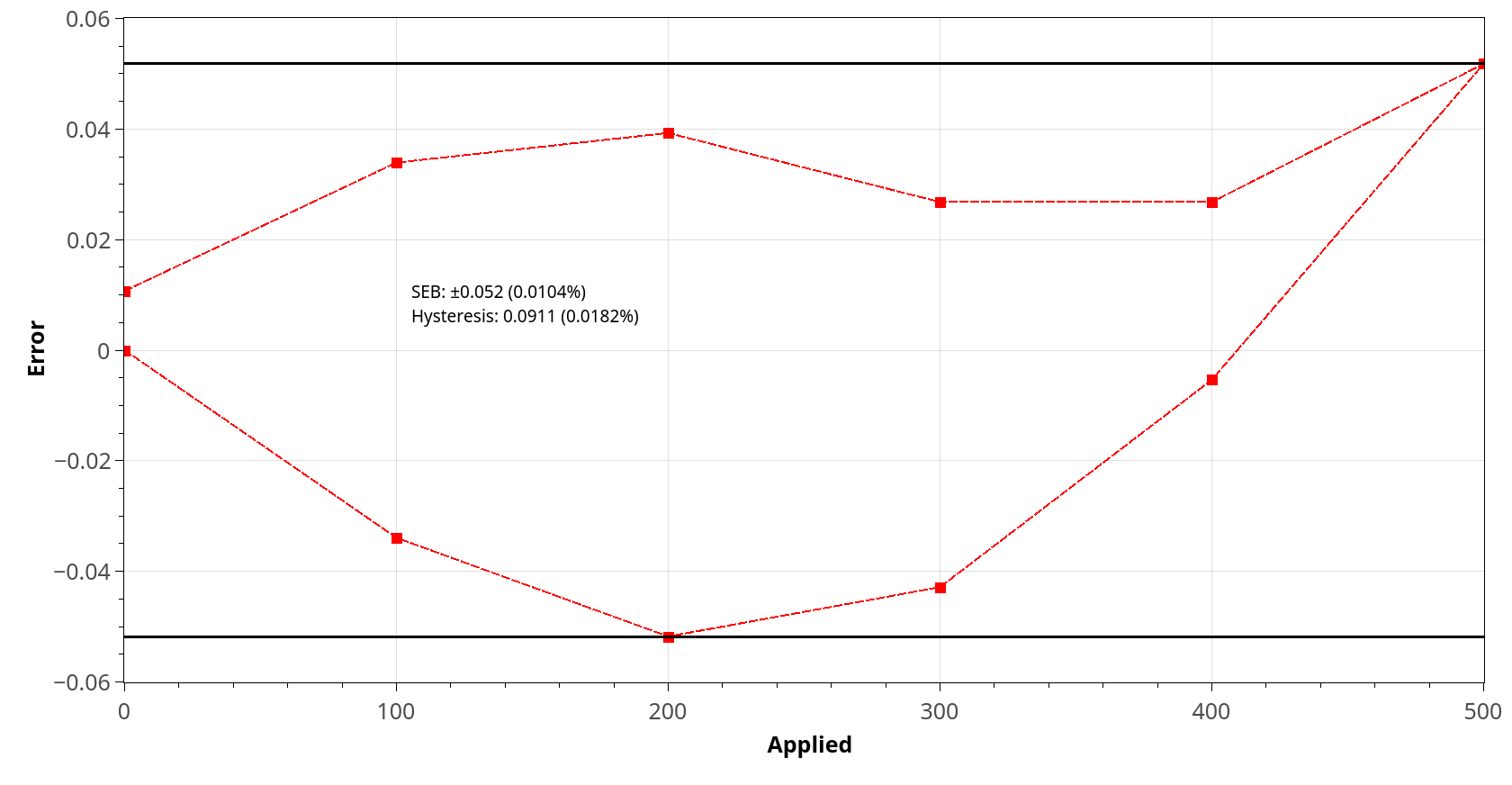
The following example makes use of the curvefit_calibration module to illustrate common measures of calibration performance.
program example
    use curvefit_calibration
    use curvefit_core, only : dp, i32
    use curvefit_regression, only : linear_least_squares
    implicit none

    ! Local Variables
    real(dp), parameter :: fullscale = 5.0d2
    real(dp), dimension(11) :: applied, output, measured, applied_copy
    real(dp) :: hyst, gain, nlin
    type(seb_results) :: s

    ! Initialization
    applied = [0.0d0, 1.0d2, 2.0d2, 3.0d2, 4.0d2, 5.0d2, 4.0d2, 3.0d2, &
        2.0d2, 1.0d2, 0.0d0]
    output = [0.0d0, 0.55983d0, 1.11975d0, 1.67982d0, 2.24005d0, &
        2.80039d0, 2.24023d0, 1.68021d0, 1.12026d0, 0.56021d0, 0.00006d0]
    applied_copy = applied

    ! Determine a suitable calibration gain (the least squares routine modifies
    ! applied; hence, the need for the copy)
    gain = linear_least_squares(output, applied_copy)

    ! Apply the calibration gain
    measured = gain * output

    ! Compute the SEB
    s = seb(applied, output, fullscale)

    ! Compute the best fit nonlinearity
    nlin = nonlinearity(applied, measured)

    ! Compute the hysteresis
    hyst = hysteresis(applied, measured)

    ! Display the results
    print '(AF9.5)', "Calibration Gain: ", gain
    print '(AF6.4)', "SEB: ", s%seb
    print '(AF7.5)', "SEB Output: ", s%output
    print '(AF7.4)', "Best Fit Nonlinearity: ", nlin
    print '(AF6.4)', "Hysteresis: ", hyst
end program
The above program yields the following data.
Calibration Gain: 178.55935
SEB: 0.0518
SEB Output: 2.80010
Best Fit Nonlinearity: -0.0582
Hysteresis: 0.0911
For visualization purposes, here is an error plot from the data in the above example. Notice, the lines drawn to illustrate the static error band.

This library can be built using CMake. For instructions on using CMake see Running CMake.
Documentation can be found here.
This library relies upon 3 other libraries.
