My homework solutions for UC Berkeley CS294: deep unsupervised learning (I did not take part in that course).
I used Tensorflow 1 and Jupyter notebooks for the first homework, but starting from the second one i will use Tensorflow 2, Python scripts instead of notebooks and store visualizations in Tensorboard.
This task is suprisingly more complex than 1.1 – I have encountered a lot of problems, and the final density plot does not look so convincing. Here are some things that are not described in the assignment / papers that I had to tweak:
- determinant of the sigmoid flow must be clipped from below with a small value like
1e-10, otherwise when a coordinate is transformed into 0 or 1 by the flow, the determinant will be 0. Although the sigmoid function never achieves 0 or 1 values, due to float precisiontf.math.sigmoid(20.)will return 1. Then the gradient of the sigmoid will be calculated as 0, and log determinant of the sigmoid flow will become negative infinity. It may be that this problem only arises because of a mistake in my implementation, and in the correct implementation the last sigmoid flow will never receive such large values. The sigmoid in the scaling part of the affine coupling flow must be bounded from below for the same reason. - the official Glow implementation uses a different formula for the affine coupling layer that limits how much the
inputs can be scaled up:
(x2 + t(x1)) * sigmoid(s(x1) + 2). This prevents the gradients from growing too large and makes the training more stable. Check out the discussion of the scale term calculation here: openai/glow#62. The+2part inside of the sigmoid pushes the initial scales into the 1 region, i guess? And away from the 0 region that would make the log determinant explode.
You can see in the density plot that all regions of high density are connected with each other through small threads of high density. Throughout all my trials I've never observed a clean separation between modes like in the density plot of the flow from the task 1.1.
Some useful resources that I read while implementing this task:
- https://github.com/MokkeMeguru/glow-realnvp-tutorial Tensorflow 2.0 + TF Probability implementations of RealNVP and Glow
- https://github.com/openai/glow/ official Tensorflow implementation of Glow. Some minor details are different from the paper or not covered there! For example, the affine coupling layer scaling thing from Task 1.2.
Have not read but plan to:
I've implemented 4 different models:
- the one suggested in the assignment, except that I used actnorm instead of data-dependent convolution initialization and added batchnorm inside the simple resnet:
chains.real_nvp chains.real_nvpwith the multiscale architecture:chains.multiscale_real_nvp- Glow:
chains.multiscale_glow chains.real_nvpbut all splits changed to 1x1 invertible convolutions:chains.glow_no_factoring
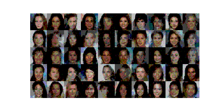
I gave all models a training time of ~4 hours, and tried to pick the parameters (number of blocks, number of steps) as large as possible so it would still fit my GPU RAM. Here is the comparison notebook with bits/dim plots and samples.


