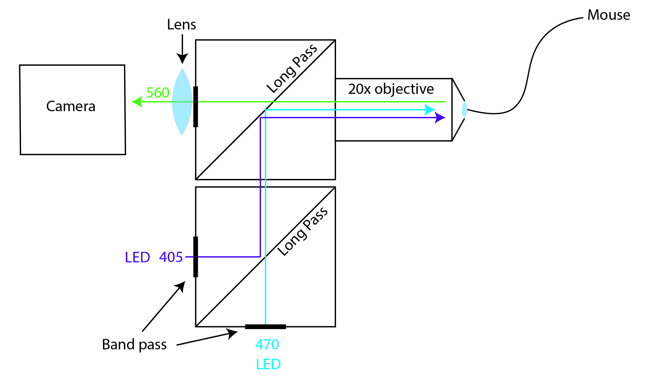
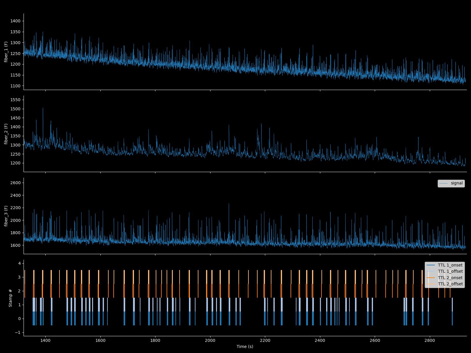
Fipster is a set of MATLAB and Python scripts used for the acquisition and analysis of fiber photometry (FIP) data on camera-based systems. It consists of:
- A wiki detailing how to build your own multi-fiber multi-color system.
- MATLAB acquisition code (FIP_acquisition) that will run the system.
- GUI-based analysis code in MATLAB (Fipster_Matlab)
- Advanced analysis code in Python (Fipster_Python)
Camera-based FIP setups can be build relatively cheap using of-the-shelf parts. They are very flexible and can be used for multi-color and multi-fiber experiments as well as experiments that combine both FIP and optogenetics. To get started have a look at the wiki and put your own setup together using the parts_list.xlsx file.
>> signal = FIP_signal('User input');
This will open a GUI where one can select a .mat file containing signal (Calcium depended, CD) and reference (405nm excitation) traces. There are currently two supported formats. One is that exported by Fipgui (Deisseroth lab) the other is the .mat files exported by the FIP_aquisition class which is also part of this toolbox. If a LogAI file with the same name is found in the same folder, this file will be imported as well. Most likely it should be straightforward to process data obtained using the neurophotometrics as well.

The MATLAB GUI is a very convenient way to quickly inspect your signals. We generally use it to look at signals right after we record them since we have MATLAB running on the acquisition computer anyway. While you can also incorporate the MATLAB code in your analysis pipeline (see "automated_workflow" for an example) we have generally moved to Python for the analysis of our experiments. While we continue to address bug fixes in the MATLAB code, we don't include new methods as we do in the Python code and therefore we've labeled it "legacy" code.
Fipster Python is actively maintained and updated. There is no GUI, but you can use matplotlib controls (both task bar as well as code) to control figure behavior. Fipster_python is completely Matplotlib and Pandas based and can be conveniently incorporated into an analysis pipeline, for instance into a Jupyter Notebook. You can import Fipster_python into your code like so:
import sys
sys.path.append('path/where/you/installed/Fipster_python/')
import Fipster as fip

# To load the data
signal = fip.FIP_signal('your/filename/here.mat')
Have a look at FIP_example.py to get a rough idea of what is possible.
You can also run Fipster_Python directly from the command line. This will present the complete dataset in a figure and make the dataset available in your workspace as an object named "signal'.
$ipython -i fipster.py ../raw_data/example_1.mat
(This will load the example data, change this to load you own data)
On Mac OS and Linux you can add Fipster_python to your .bashrc or .zshrc as an alias to conveniently load FIP data from anywhere:
alias fipster="ipython -i path/where/you/installed/Fipster_python/Fipster.py"
There will be a detailed tutorial soon. But for now you should be able to get detailed instruction on the included method using the "help" method or by reading the docstrings of the code. For instance:
dir(signal) # Will print a list of properties and methods
help(signal) # Will print available docstrings of methods
help(signal.plot) # Will print docstring of the 'plot' method
help(signal.derive_timestamps) # Will print docstring of the "derive_timestamps" method
# etc..Fipster python allows for auROC normalization, which has a lot of advantaged over z-score normalization for trial-based assays. The idea is from Cohen et al. Nature 2012. Specifically, it is in figure S1 of that paper.

