This report describes the usage of SegNet and U-Net architechtures for medical image segmentation.
We divide the article into the following parts
The dataset contains Chest X-Ray images. We use this dataset to perform a lung segmentation.
The dataset can be found here
Structure:
We make the following structure of the given data set:


The Montgomery dataset contains images from the Department of Health and Human Services, Montgomery County, Maryland, USA. The dataset consists of
138 CXRs, including 80 normal patients and 58 patients with manifested tuberculosis (TB). The CXR images are 12-bit gray-scale images of dimension 4020 × 4892 or 4892 × 4020 . Only the two lung masks annotations are available which were combined to a single image in order to make it easy for the network to learn the task of segmentation (Fig 1).To make all images of symmetric dimensions we padded the pictures to the maximum dimension in their height or width such that images are of 4892 x 4892, this is done to preserve the aspect ratio of CXR while resizing. We scale all images to 1024 x 1024 pixels, which retains sufficient visual details for vascular structures in the lung fields and this could be the maximum size that could be accommodated in, along with U-Net in Graphics Processing Unit (GPU). We scaled all pixel values to 0-1 . Data augmentation was applied by flipping around the vertical axis and adding gaussian noise with mean 0 and a variance of 0.01. Also rotation about the centre to subtle angles of 5-10 degrees during runtime were performed to make the model more robust.

SegNet has an encoder network and a corresponding decoder network, followed by a final pixelwise classification layer. This architecture is illustrated in the above figure. The encoder network consists of 13 convolutional layers which correspond to the first 13 convolutional layers in the VGG16 network designed for object classification. We can therefore initialize the training process from weights trained for classification on large datasets. We can also discard the fully connected layers in favour of retaining higher resolution feature maps at the deepest encoder output. This also reduces the number of parameters in the SegNet encoder network significantly (from 134M to 14.7M) as compared to other recent architectures. Each encoder layer has a corresponding decoder layer and hence the decoder network has 13 layers. The final decoder output is fed to a multi-class soft-max classifier or for a binary classification task, to a sigmoid activation function to produce class probabilities for each pixel independently. Each encoder in the encoder network performs convolution with a filter bank to produce a set of feature maps. These are then batch normalized. Then an element-wise rectified- linear non-linearity (ReLU) max (0, x) is applied. Following that, max-pooling with a 2 × 2 window and stride 2 (non-overlapping window) is performed and the resulting output is sub-sampled by a factor of 2. Max-pooling is used to achieve translation invariance over small spatial shifts in the input image. Sub-sampling results in a large input image context (spatial window) for each pixel in the feature map. While several layers of max-pooling and sub-sampling can achieve more translation invariance for robust classification correspondingly there is a loss of spatial resolution of the feature maps. The increasingly lossy (boundary detail) image representation is not beneficial for segmentation where boundary delineation is vital.
U-Net (O. Ronneberger and P.Fischer and T. Brox) is a network that is used to train on medical images to segment the image according to a given mask. The network architecture is illustrated in Figure 1. It consists of a contracting path (left side) and an expansive path (right side). The contracting path follows the typical architecture of a convolutional network. It consists of the repeated application of two 3x3 convolutions (padded convolutions in this case), each followed by a rectified linear unit (ReLU) and a 2x2 max pooling operation with stride 2 for downsampling. At each downsampling step we double the number of feature channels. Every step in the expansive path consists of an upsampling of the feature map followed by a 2x2 convolution (“bilinear interpolation”) that halves the number of feature channels, a concatenation with the corresponding feature map from the contracting path, and two 3x3 convolutions, each followed by a ReLU. At the final layer a 1x1 convolution is used to map each 64-component feature vector to the desired number of classes. In total the network has 23 convolutional layers. It is important to select the input image size such that all 2x2 max-pooling operations are applied to a layer with an even x- and y-size.
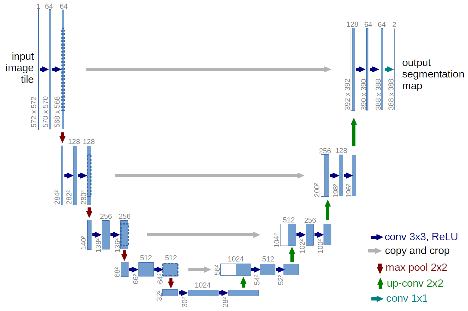
We input the images to the network, which is first passed through the network encoder, this outputs a 1024 channel feature map as show in the above figure. This feature map is then upsampled back to the orignal size using upsampling(bilinear Interpolation). At each upsampling layer, a skip connection to its corresponding layer in the encoder, the channels from both layers are concatenated and this is used as input for the next upsampling layer.
Finally, on the final layer, sigmoid activation is applied and the resulting feature map is then thesholded at 0.5 and which is then the segmented image.
We use two loss functions here, viz. Binary Cross Entropy and Dice loss
Cross-entropy loss, or log loss, measures the performance of a classification model whose output is a probability value between 0 and 1. Cross-entropy loss increases as the predicted probability diverges from the actual label. So predicting a probability of .012 when the actual observation label is 1 would be bad and result in a high loss value. A perfect model would have a log loss of 0.
It is defined mathematically as
In binary classification, where the number of classes
The dice coefficient loss is used to measure the intersection over union of the output and target image.
Mathematically, Dice Score is
and the corresponding loss is
The dice loss is defined in code as :
class SoftDiceLoss(nn.Module):
    def __init__(self, weight=None, size_average=True):
        super(SoftDiceLoss, self).__init__()

    def forward(self, logits, targets):
        smooth = 1
        num = targets.size(0)
        probs = F.sigmoid(logits)
        m1 = probs.view(num, -1)
        m2 = targets.view(num, -1)
        intersection = (m1 * m2)

        score = 2. * (intersection.sum(1) + smooth) / (m1.sum(1) + m2.sum(1) + smooth)
        score = 1 - score.sum() / num
        return score
The formula below calculates the measure of overlap after inverting the image or in this case taking the complement.
Mathematically, Inverted Dice Score is
class SoftInvDiceLoss(nn.Module):
    def __init__(self, weight=None, size_average=True):
        super(SoftDiceLoss, self).__init__()

    def forward(self, logits, targets):
        smooth = 1
        num = targets.size(0)
        probs = F.sigmoid(logits)
        m1 = probs.view(num, -1)
        m2 = targets.view(num, -1)
        m1, m2 = 1.-m1, 1.-m2
        intersection = (m1 * m2)

        score = 2. * (intersection.sum(1) + smooth) / (m1.sum(1) + m2.sum(1) + smooth)
        score = 1 - score.sum() / num
        return score
NOTE: The reason why intersection is implemented as a multiplication and the cardinality as
sum()on axis 1 (each 3 channels sum) is because predictions and targets are one-hot encoded vectors
| Architecture | Loss | Validation Scores | Validation Scores | Test Scores | Test Scores |
|---|---|---|---|---|---|
| mIoU | mDice | mIoU | mDice | ||
| U-Net | BCE | 0.9403 | 0.9692 | - | - |
| U-Net | BCE+DCL | 0.9426 | 0.9704 | - | - |
| U-Net | BCE+DCL+IDCL | 0.9665 | 0.9829 | 0.9295 | 0.9623 |
| SegNet | BCE | 0.8867 | 0.9396 | - | - |
| SegNet | BCE+DCL | 0.9011 | 0.9477 | - | - |
| SegNet | BCE+DCL+IDCL | 0.9234 | 0.9600 | 0.8731 | 0.9293 |
The results with this network are good, and the some of the best ones are shown here
To be added shortly.