sdetorus

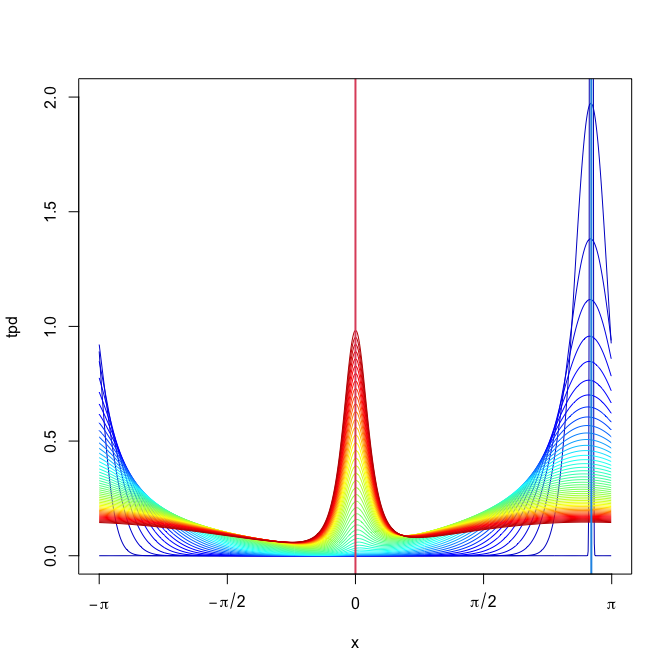
Transition probability density of the Langevin diffusion guided by the “sdetorus” density

Overview

This library provides statistical tools for estimation of toroidal diffusions. It is the package companion for the paper Langevin diffusions on the torus: estimation and applications (García-Portugués et al., 2019).

Install

Get the released version from CRAN:

# Install the package
install.packages("sdetorus")

# Load package
library(sdetorus)

Alternatively, get the latest version from GitHub:

# Install the package
library(devtools)
Sys.setenv("PKG_CXXFLAGS" = "-std=c++11")
Sys.setenv("PKG_LIBS" = "-llapack")
install_github("egarpor/sdetorus")

# Load package
library(sdetorus)

Usage

Example 1: simulation of diffusion trajectories

# Load package
library(sdetorus)

## vM diffusion in 1D

# Initial points
nx0 <- 50
x0 <- seq(-pi, pi, l = nx0 + 1)[-(nx0 + 1)]
plot(rep(0, nx0), x0, pch = 16, col = rainbow(nx0), xlim = c(0, 1),
     xlab = expression(t), ylab = expression(Theta[t]), axes = FALSE)
torusAxis(2)
axis(1)

# Trajectories of the vM diffusion
N <- 100
mu <- 0
set.seed(12345678)
samp <- euler1D(x0 = x0, mu = mu, alpha = 3, sigma = 1, N = N,
                delta = 0.01, type = 2)
abline(h = mu)
tt <- seq(0, 1, l = N + 1)
for (i in 1:nx0) linesCirc(tt, samp[i, ], col = rainbow(nx0)[i])
points(rep(1, nx0), samp[, N + 1], pch = 16, col = rainbow(nx0))

## WN diffusion in 2D

# Initial points
nx0 <- 10
x0 <- seq(-pi, pi, l = nx0)
x0 <- as.matrix(expand.grid(x0, x0))
nx0 <- nx0^2
plot(x0[, 1], x0[, 2], xlim = c(-pi, pi), ylim = c(-pi, pi), pch = 16,
     col = rainbow(nx0), xlab = expression(Theta[list(1,t)]),
     ylab = expression(Theta[list(2,t)]), axes = FALSE)
torusAxis()

# Trajectories of the WN diffusion
N <- 100
set.seed(12345678)
samp <- euler2D(x0 = x0, mu = c(0, 0), A = rbind(2:1, 1:2),
                sigma = c(1, 1), N = N, delta = 0.01, type = 1)
for (i in 1:nx0) linesTorus(samp[i, 1, ], samp[i, 2, ],
                            col = rainbow(nx0, alpha = 0.5)[i])

Example 2: computation of transition probability densities

# Load package
library(sdetorus)

## Cauchy diffusion in 1D

# Drift
Mx <- 1e3
x <- seq(-pi, pi, l = Mx + 1)[-c(Mx + 1)]
mu <- 0
b <- driftJp(x = x, alpha = 1, mu = mu, psi = -1)

# Squared diffusion coefficient
sigma2 <- rep(1, Mx)

# Initial condition concentrated at x0
x0 <- pi - 0.25
sdInitial <- 0.01
u0 <- cbind(dWn1D(x = x, mu = x0, sigma = sdInitial))
periodicTrapRule1D(u0)
#> [1] 1

# Tpd for times t = 0.0, 0.1, 0.2, ..., 5.0
N <- 5e3
n <- seq(0, N, by = 100)
tpd <- crankNicolson1D(u0 = u0, b = b, sigma2 = sigma2, N = n, deltat = 2 / N,
                       Mx = Mx, deltax = 2 * pi / Mx)
matplot(x, tpd, type = "l", col = matlab.like.colorRamps(length(n), two = TRUE),
        lty = 1, ylim = c(0, 2), axes = FALSE)
abline(v = c(x0, mu), col = c(4, 2), lwd = 2)
torusAxis(1)
axis(2)

## WN diffusion in 2D

# Function for computing and plotting a tpd
plotTpd <- function(t) {

  Mx <- 150
  tpd <- dTpdPde2D(Mx = Mx, My = Mx, x0 = c(pi / 2, -pi), t = t,
                   alpha = c(1, 1, 0), mu = c(0, 0), sigma = c(2, 1),
                   type = "WN", Mt = ceiling(1e2 * t), sdInitial = 0.1)
  x <- seq(-pi, pi, l = Mx)
  plotSurface2D(x = x, y = x, z = pmin(tpd, 0.25), axes = FALSE,
                xlab = expression(theta[1]), ylab = expression(theta[2]),
                main = paste("t =", t), levels = seq(0, 0.25, l = 20))
  torusAxis()
  points(c(0, pi / 2, pi / 2), c(0, -pi, pi), pch = 16, cex = 1)

}

# Tpd at different times
par(mfrow = c(2, 2))
plotTpd(t = 0.2)
plotTpd(t = 0.5)
plotTpd(t = 1.0)
plotTpd(t = 3.0)

Example 3: approximate maximum likelihood estimation in 1D

# Load package
library(sdetorus)

## WN diffusion in 1D

# Sample
set.seed(12345678)
N <- 500
delta <- 0.1
samp <- rTrajWn1D(x0 = 0, alpha = 0.5, mu = pi, sigma = 1, N = N, delta = delta)
tt <- seq(0, N * delta, by = delta)
plot(tt, samp, type = "n", ylim = c(-pi, pi), xlab = expression(t),
     ylab = expression(Theta[t]), axes = FALSE)
linesCirc(x = tt, y = samp)
axis(1)
torusAxis(2)

# Drift and diffusion
b <- function(x, pars) driftWn1D(x = x, alpha = pars[1], mu = pars[2],
                                 sigma = pars[3])
b1 <- function(x, pars, h = 1e-4) {
  l <- length(x)
  res <- driftWn1D(x = c(x + h, x, x - h), alpha = pars[1], mu = pars[2],
                   sigma = pars[3])
  drop(res[1:l] - 2 * res[(l + 1):(2 * l)] + res[(2 * l + 1):(3 * l)])/(h^2)
}
sigma2 <- function(x, pars) rep(pars[3]^2, length(x))

# Common optimization parameters
start <- 1:3
low <- c(0, -pi, 0)
up <- c(100, pi, 100)

# MLE by numerical solution of PDE
est1 <- mlePde1D(data = samp, delta = delta, b = b, sigma2 = sigma2, Mx = 5e2,
                 sdInitial = 0.05, start = start, lower = low, upper = up)

# Euler pseudo-likelihood
est2 <- psMle(data = samp, delta = delta, method = "E", b = b, sigma2 = sigma2,
              start = start, lower = low, upper = up)

# Shoji--Ozaki pseudo-likelihood
est3 <- psMle(data = samp, delta = delta, method = "SO", b = b, b1 = b1,
              sigma2 = sigma2, start = start, lower = low, upper = up)

# Approximate MLE based on the WOU process
est4 <- approxMleWn1D(data = samp, delta = delta, start = start, lower = low,
                      upper = up)

# Comparison
est1$par
#> [1]  0.5310225 -2.9645313  1.0423494
est2$par
#> [1]  0.4887261 -3.0923169  1.0340890
est3$par
#> [1] 0.3088016 2.7632043 1.0394086
est4$par
#> [1]  0.514412 -2.873781  1.060543

Replicability of García-Portugués et al. (2019)

The directories /MD and /simulation in the data-langevintorus repository contain the scripts used in the empirical analyses of the aforementioned paper, as well as their .RData outputs.

References

García-Portugués, E., Sørensen, M., Mardia, K. V., and Hamelryck, T. (2019). Langevin diffusions on the torus: estimation and applications. Statistics and Computing, 29(2):1–22. doi:10.1007/s11222-017-9790-2.

egarpor / sdetorus