bmaxdk / path-planning

Path Planning

path-planning

Path Planning

Approaches to Path Planning

Three different approaches:

• Discrete (or combinatorial) path planning
• Sample-based path planning
• Probabilistic path planning

Discrete Planning

Discretize the robot’s workspace into a connected graph, and apply a graph-search algorithm to calculate the best path. It is very computationall very expensive. Therefore, it is best suited for low-dimensional problems. For high-dimensional problems, sample-based path planning is a more appropriate approach.

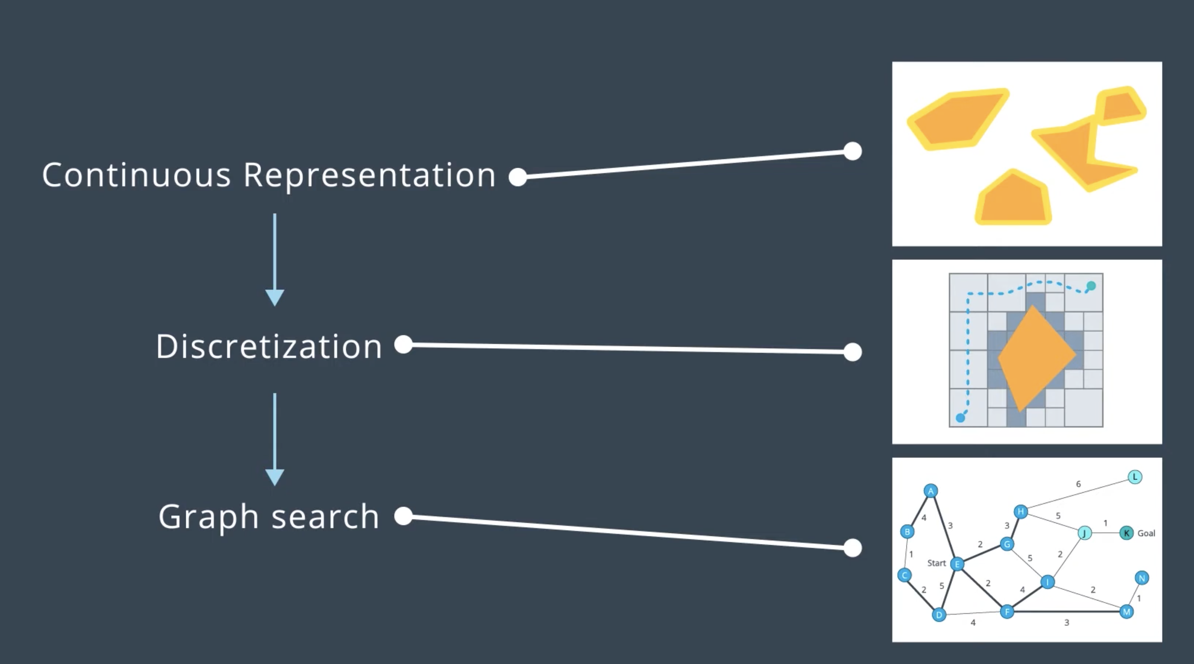
• Develop a convenient continuous representation. This can be done by representing the problem space as the configuration space (C space). C space takes into account the geometry of the robot and makes it easier to apply discrete search algorithms.
• Discretization. The configuration space must be discretized into a representation that is more easily manipulated by algorithms.
• Graph Search. The descretized space is represented by a graph to use search algorithm. Find the best path from the start node to the goal node.

Continuous Representation

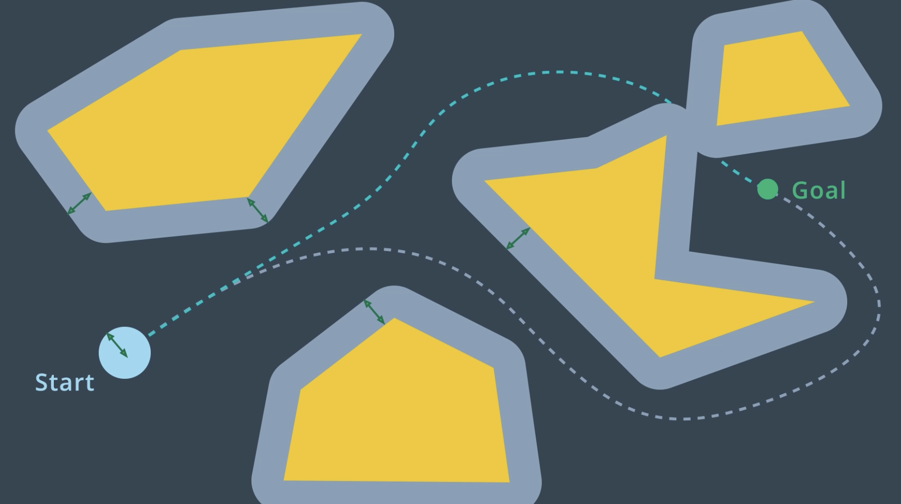
Find a curved or piece wise linear path connecting the robot start pose to the goal pose that does not collied with any obstacles. 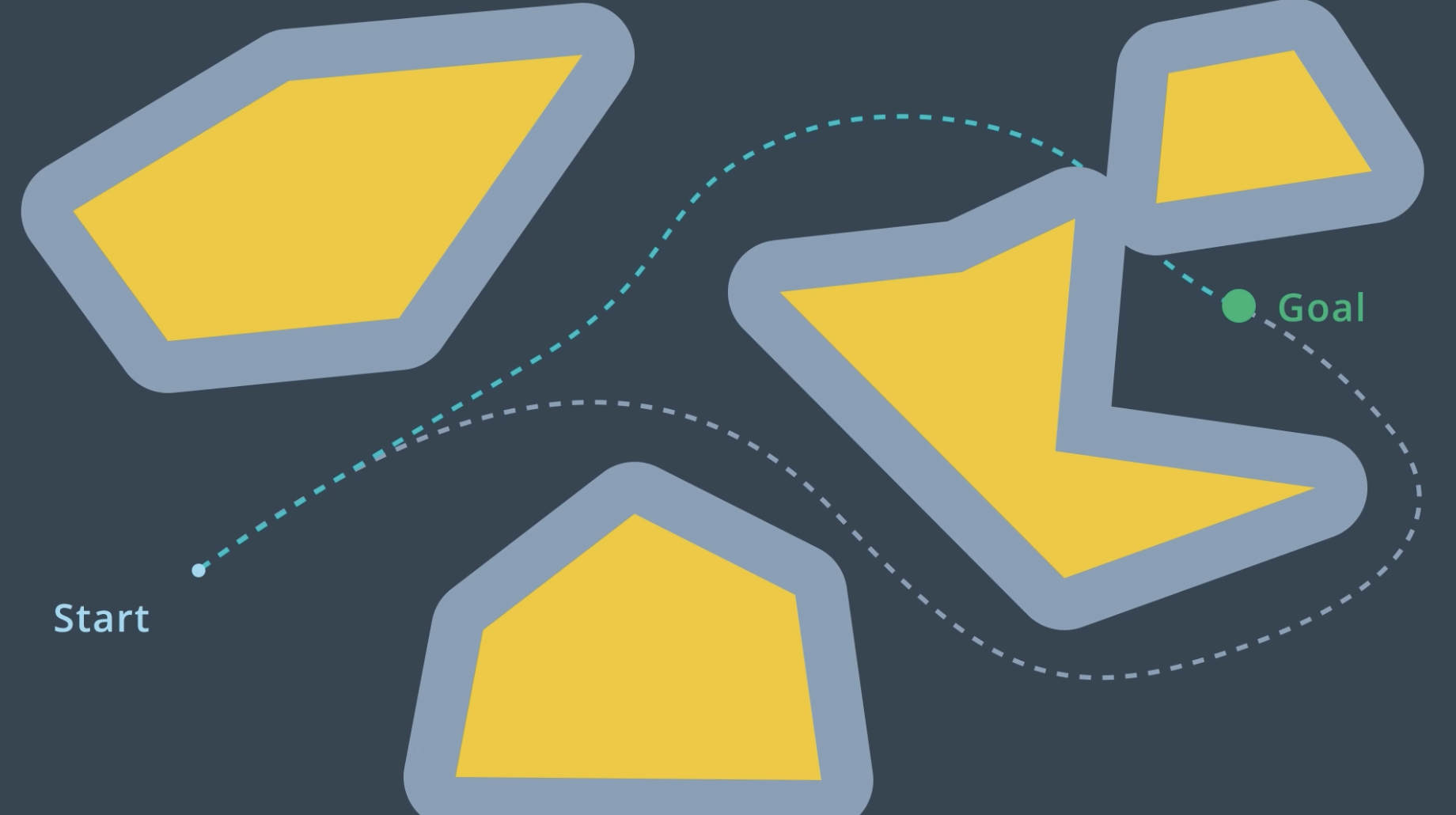Inflate every single obstacle by the radius of the robot and then treat the robot as a point.

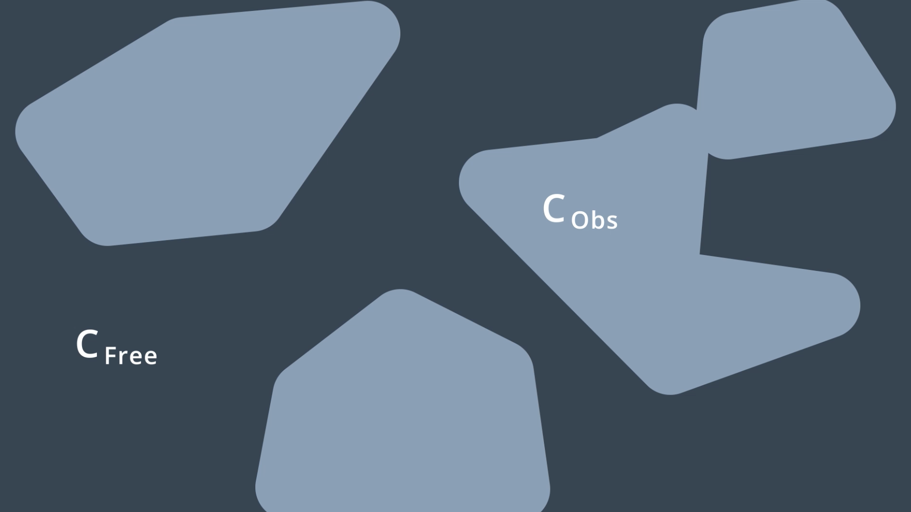This kinds of environment is the configuration space(C space). A configuration space is a set of all robot poses. The C space is divided into $C_{free}$ and $C_{obstacle}$. $C_{obstacle}$ is the compliment to $C_{free}$ representing the set of robot pauses that are in collision with obstacles or walls.

Minkowski Sum

Let P and R be two sets in $\mathbb{R}_{2}$

$P \oplus R$ = {p+r | p $\in$ P $\wedge$ r $\in$ R}

where p+r = ($p_{x}+r_{x}, p_{y}+r_{y}$)

The Minkowski sum is a mathematical property that can be used to compute the configuration space given an obstacle geometry and robot geometry. To create the configuration space, the Minkowski sum is calculated in such a way for every obstacle in the workspace. The image below shows three configuration spaces created from a single workspace with three different sized robots. 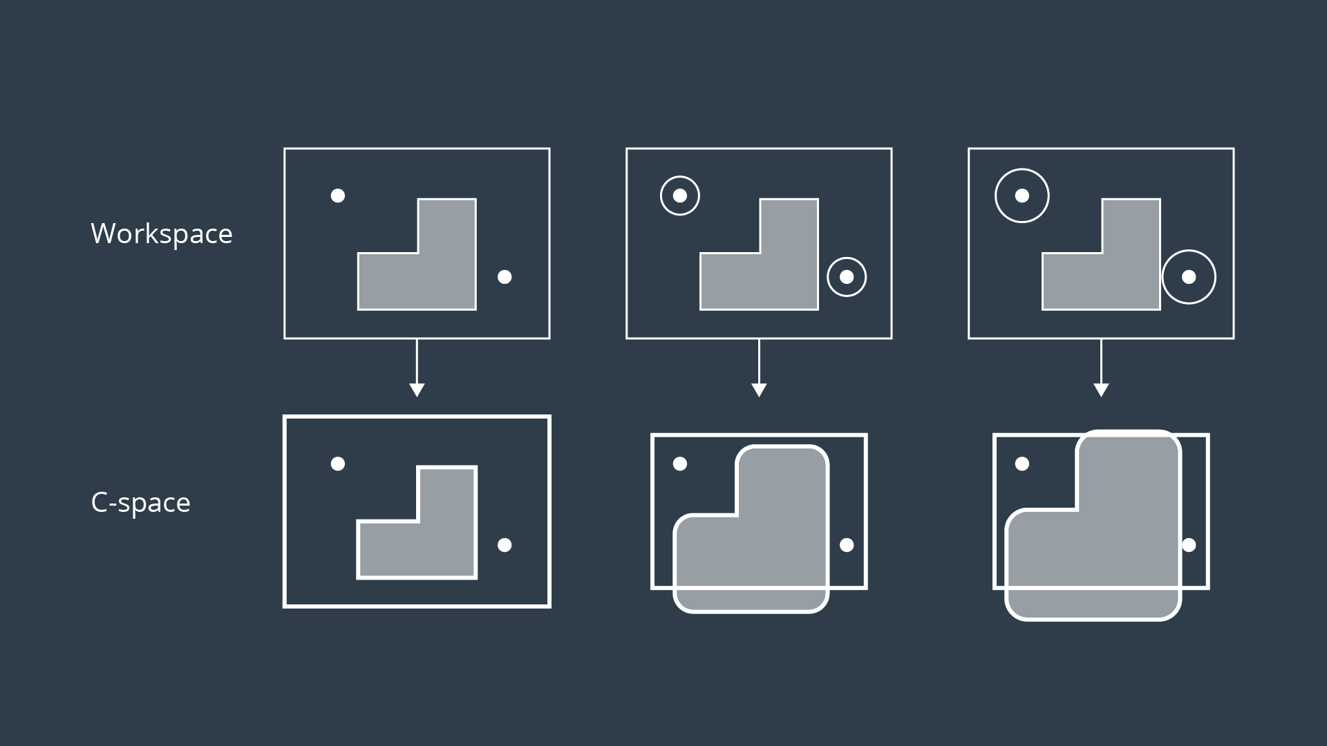For convex polygons, computing the convolution is trivial and can be done in linear time - however for non-convex polygons (i.e. ones with gaps or holes present), the computation is much more expensive. Plot check RoboND-MinkowskiSum

3D Configuration Space

Configuration space changes depending on the orientation of the robot. The apporpriate way to represent this in the configuration space is to add a dimension. The x-y plane would continue to represent the translation of the robot in the workspace, while the vertical axis would represent rotation of the robot.

The dimension of the configuration space is equal to the number of degrees of freedom that the robot has. While a 2D configuration space was able to represent the x- and y-translation of the robot, a third dimension is required to represent the rotation of the robot. A three-dimensional configuration space can be generated by stacking two-dimensional configuration spaces as layers. 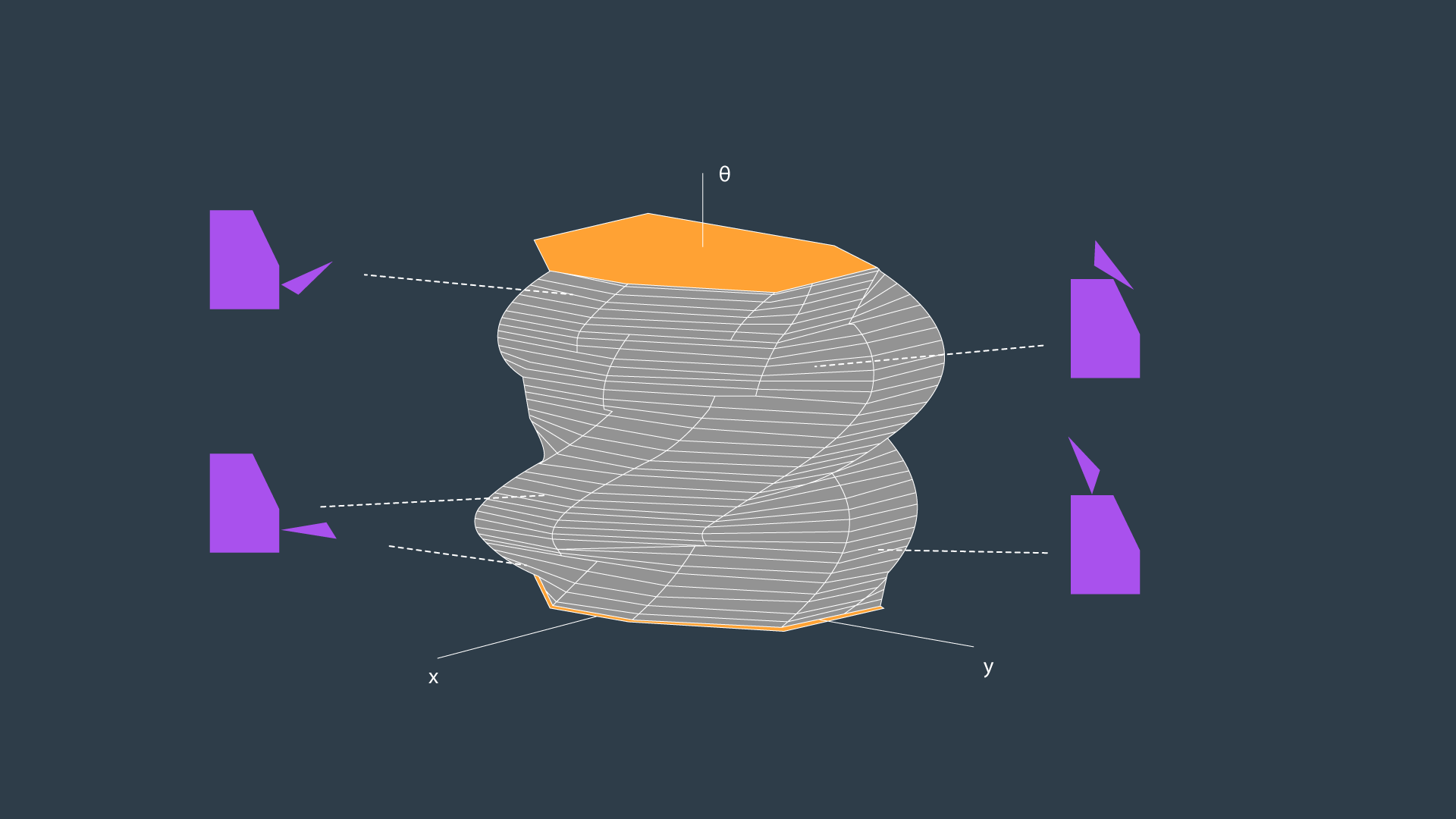The image above displays the configuration space for a triangular robot that is able to translate in two dimensions as well as rotate about its z-axis. Configuration Space Visualization

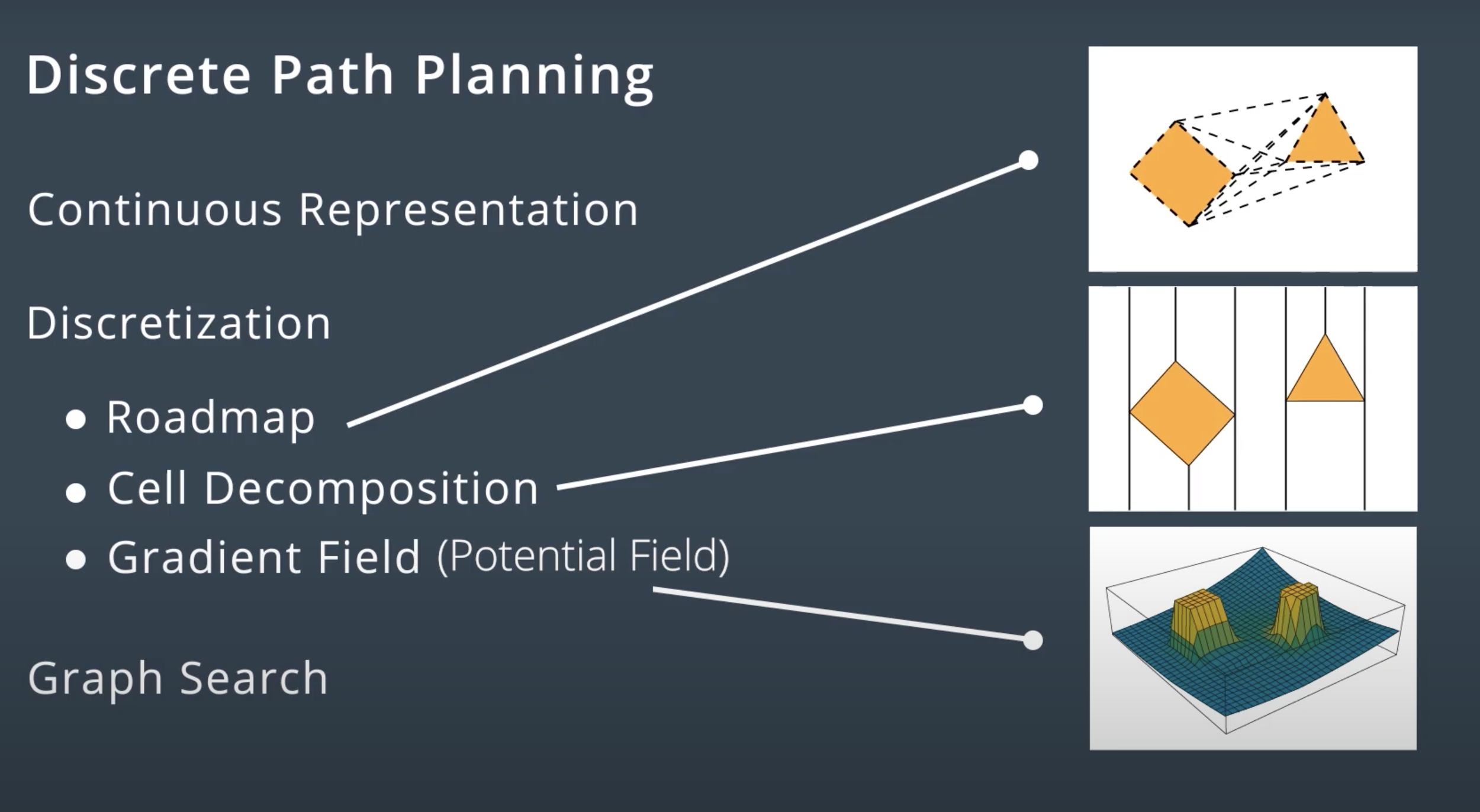
Roadmap

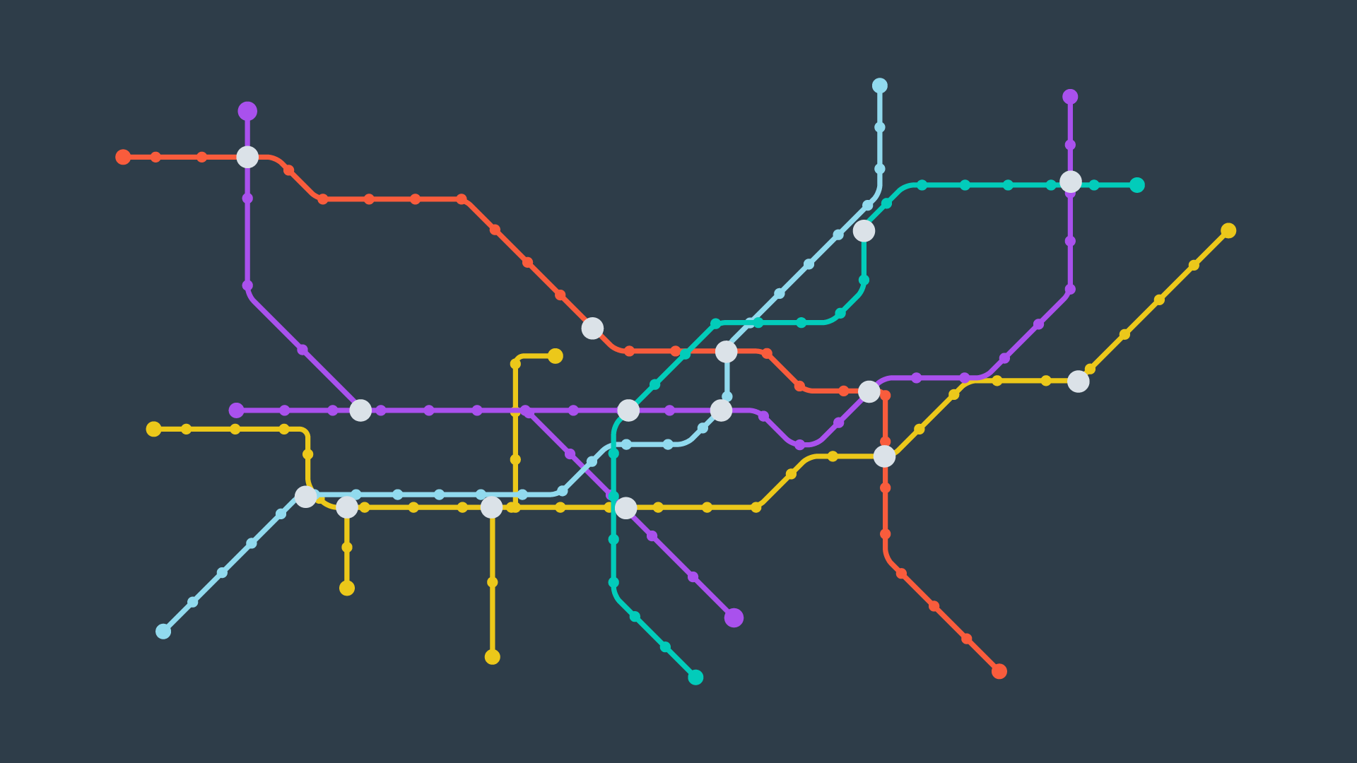
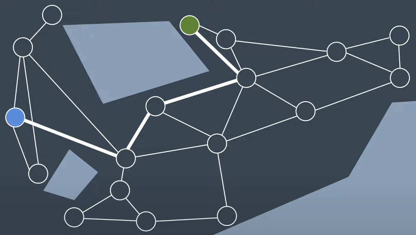
These methods represent the configuration space using a simple connected graph - similar to how a city can be represented by a metro map.

Roadmap methods are typically implemented in two phases:

• The construction phase builds up a graph from a continuous representation of the space. This phase usually takes a significant amount of time and effort, but the resultant graph can be used for multiple queries with minimal modifications.
• The query phase evaluates the graph to find a path from a start location to a goal location. This is done with the help of a search algorithm.

Visibility Graph

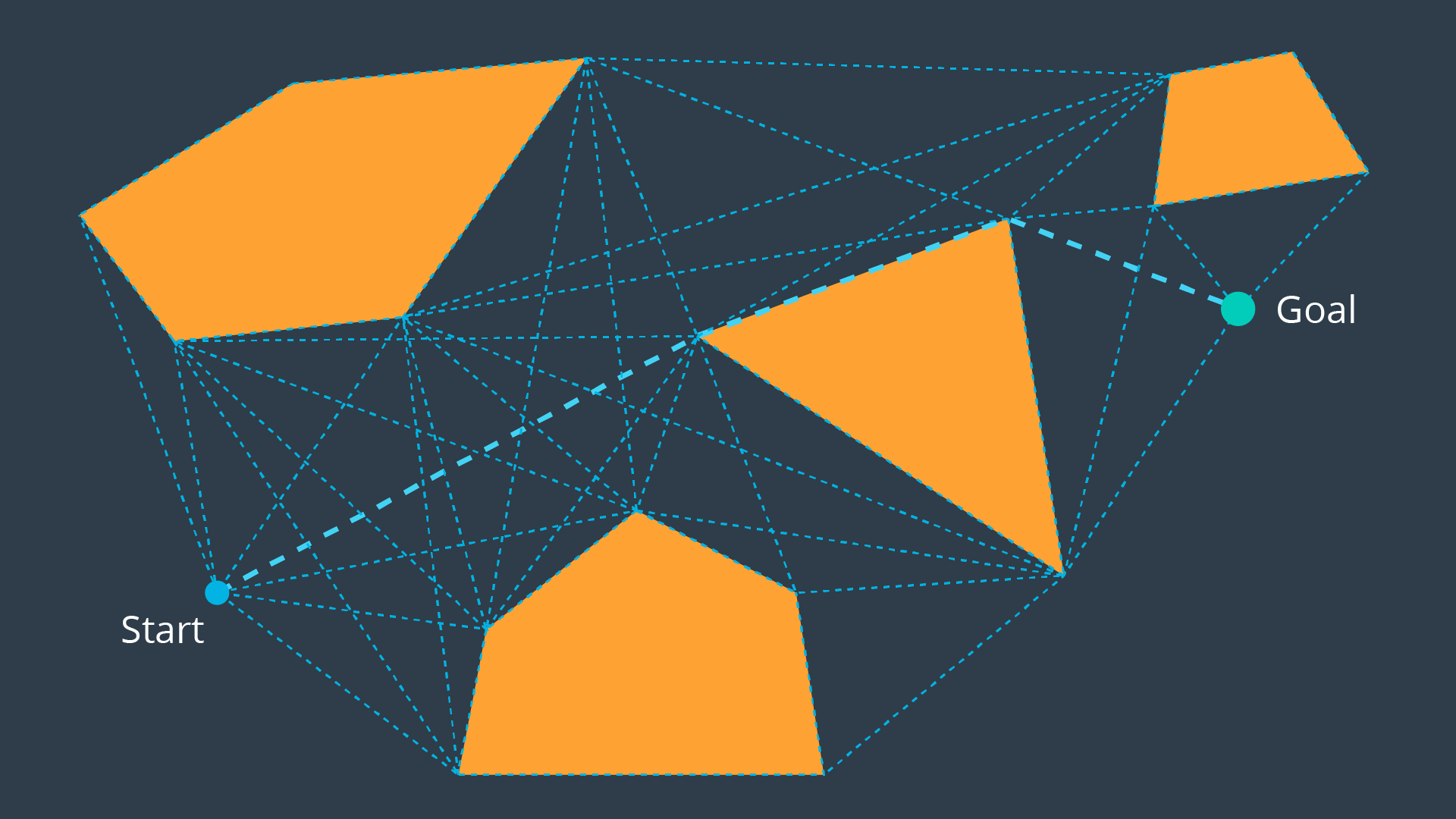
The Visibility Graph builds a roadmap by connecting the start node, all of the obstacles’ vertices, and goal node to each other - except those that would result in collisions with obstacles. The Visibility Graph has its name for a reason - it connects every node to all other nodes that are ‘visible’ from its location.

• Nodes: Start, Goal, and all obstacle vertices.
• Edges: An edge between two nodes that does not intersect an obstacle, including obstacle edges.

The motivation for building Visibility Graphs is that the shortest path from the start node to the goal node will be a piecewise linear path that bends only at the obstacles’ vertices. This makes sense intuitively - the path would want to hug the obstacles’ corners as tightly as possible, as not to add any additional length. In certain applications, such as animation or path planning for video games, this is acceptable. However the uncertainty of real-world robot localization makes this method impractical. [Complete and optimal path]

Voronoi Diagram

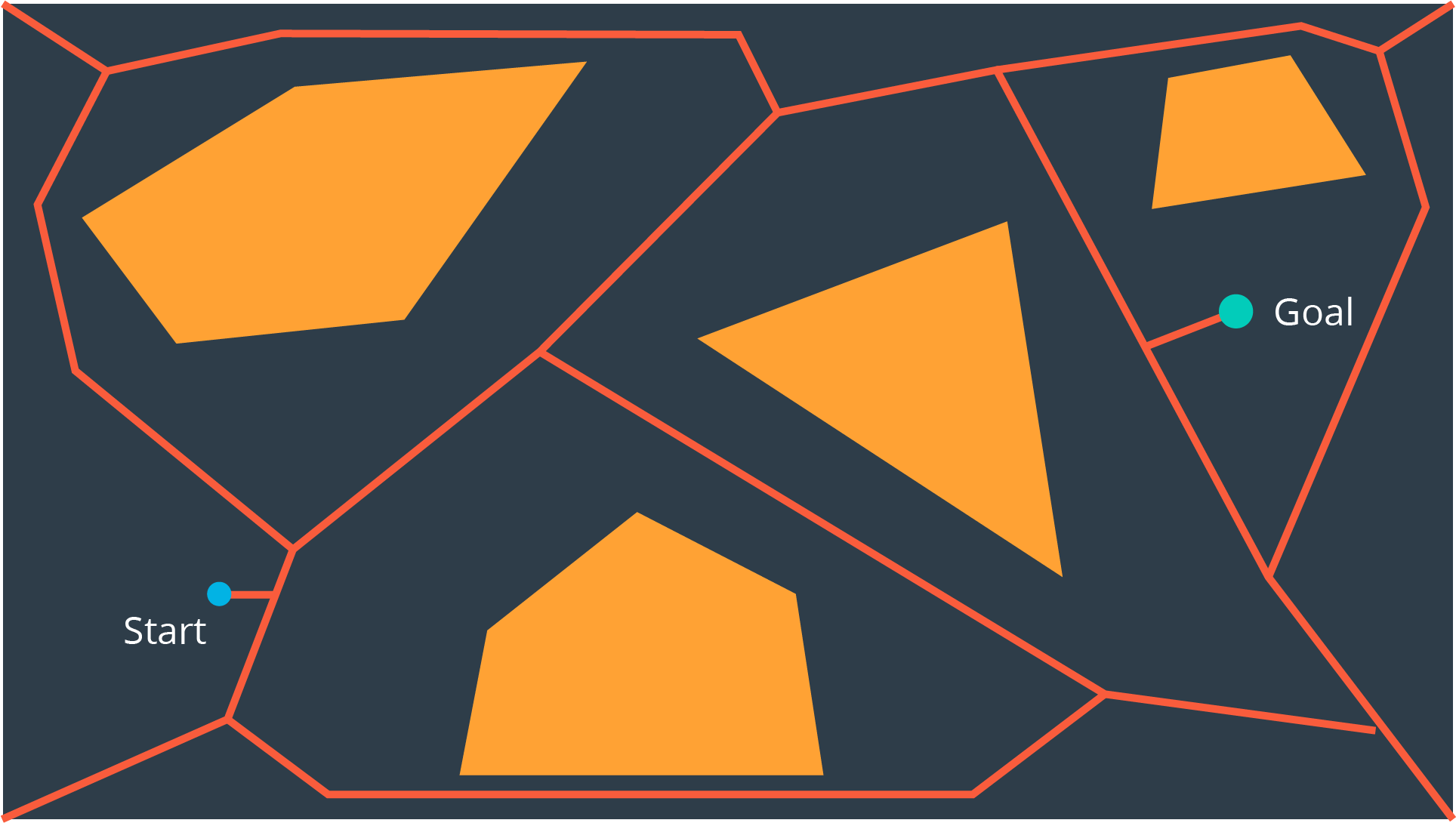
Another discretization method that generates a roadmap is called the Voronoi Diagram. Unlike the visibility graph method which generates the shortest paths, Voronoi Diagrams maximize clearance between obstacles. A Voronoi Diagram is a graph whose edges bisect the free space in between obstacles. Every edge lies equidistant from each obstacle around it - with the greatest amount of clearance possible.

Once a Voronoi Diagram is constructed for a workspace, it can be used for multiple queries. Start and goal nodes can be connected into the graph by constructing the paths from the nodes to the edge closest to each of them.

Every edge will either be a straight line, if it lies between the edges of two obstacles, or it will be a quadratic, if it passes by the vertex of an obstacle. [Complete path]

Cell Decomposition

Another discretization method that can be used to convert a configuration space into a representation that can easily be explored by a search algorithm is cell decomposition. Cell decomposition divides the space into discrete cells, where each cell is a node and adjacent cells are connected with edges. There are two distinct types of cell decomposition:

• Exact Cell Decomposition
• Approximate Cell Decomposition.

Exact Cell Decomposition

Exact cell decomposition divides the space into non-overlapping cells. This is commonly done by breaking up the space into triangles and trapezoids, which can be accomplished by adding vertical line segments at every obstacle’s vertex. 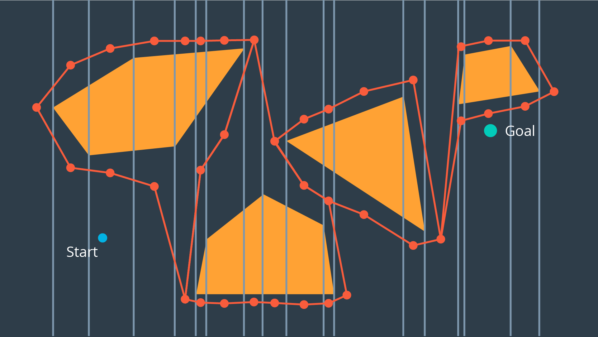Once a space has been decomposed, the resultant graph can be used to search for the shortest path from start to goal. 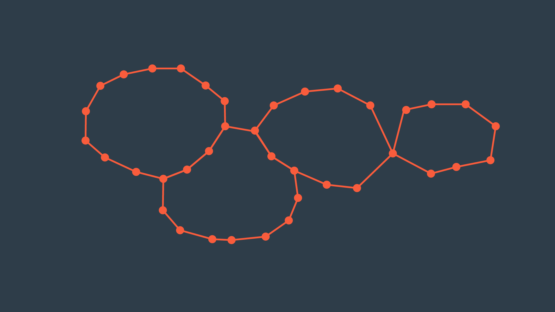Exact cell decomposition is elegant because of its precision and completeness. Every cell is either ‘full’, meaning it is completely occupied by an obstacle, or it is ‘empty’, meaning it is free. And the union of all cells exactly represents the configuration space. If a path exists from start to goal, the resultant graph will contain it.

To implement exact cell decomposition, the algorithm must order all obstacle vertices along the x-axis, and then for every vertex determine whether a new cell must be created or whether two cells should be merged together. Such an algorithm is called the Plane Sweep algorithm.

Approximate Cell Decomposition

Approximate cell decomposition divides a configuration space into discrete cells of simple, regular shapes - such as rectangles and squares (or their multidimensional equivalents). Aside from simplifying the computation of the cells, this method also supports hierarchical decomposition of space.

Simple Decomposition

A 2-dimensional configuration space can be decomposed into a grid of rectangular cells. Then, each cell could be marked full or empty, as before. A search algorithm can then look for a sequence of free cells to connect the start node to the goal node.

Such a method is more efficient than exact cell decomposition, but it loses its completeness. It is possible that a particular configuration space contains a feasible path, but the resolution of the cells results in some of the cells encompassing the path to be marked ‘full’ due to the presence of obstacles. A cell will be marked ‘full’ whether 99% of the space is occupied by an obstacle or a mere 1%. Evidently, this is not practical.

Iterative Decomposition

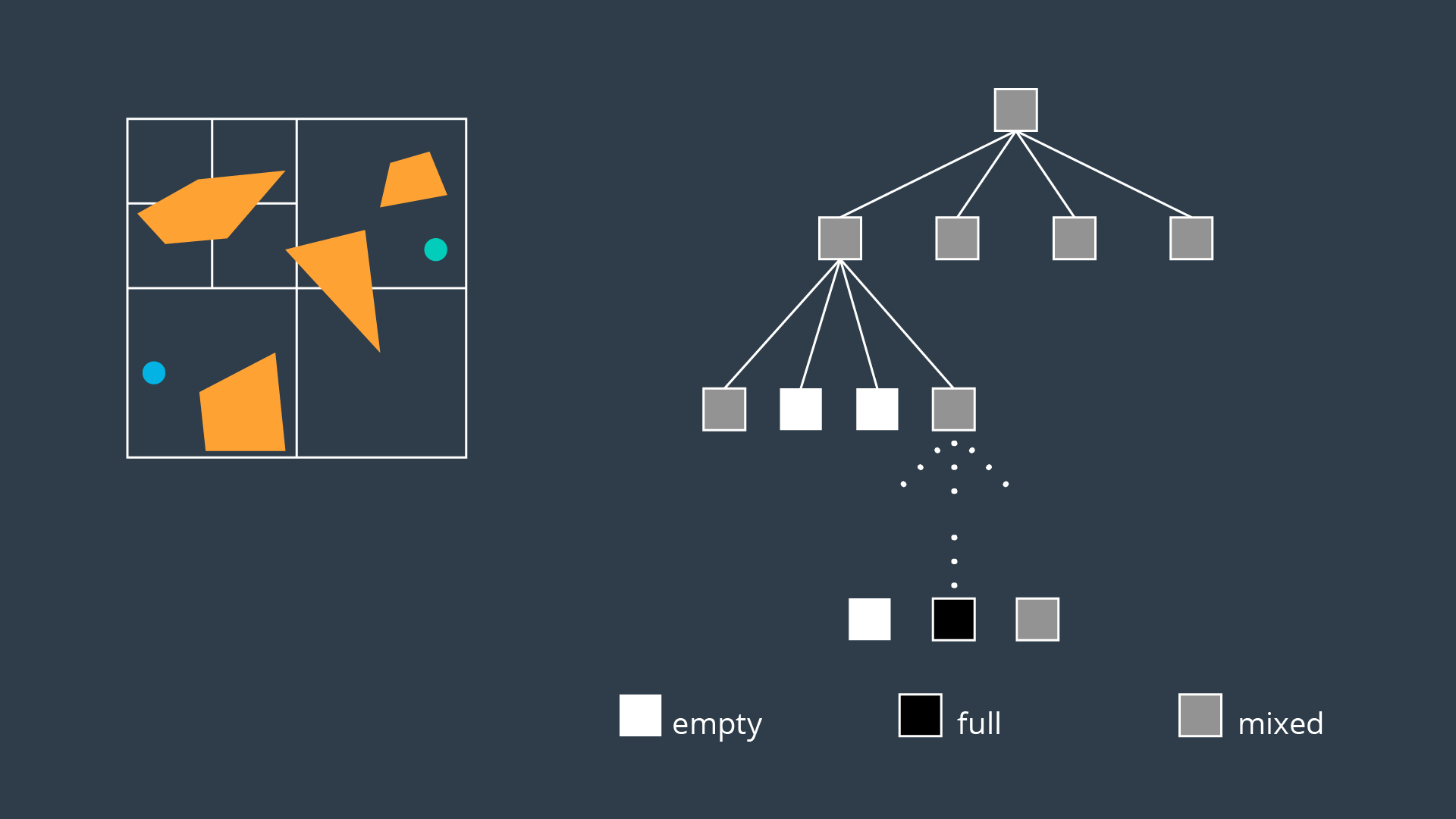
An alternate method of partitioning a space into simple cells exists. Instead of immediately decomposing the space into small cells of equal size, the method recursively decomposes a space into four quadrants. Each quadrant is marked full, empty, or a new label called ‘mixed’ - used to represent cells that are somewhat occupied by an obstacle, but also contain some free space. If a sequence of free cells cannot be found from start to goal, then the mixed cells will be further decomposed into another four quadrants. Through this process, more free cells will emerge, eventually revealing a path if one exists.

The 2-dimensional implementation of this method is called quadtree decomposition.

Algorithm

The algorithm behind approximate cell decomposition is much simpler than the exact cell decomposition algorithm.

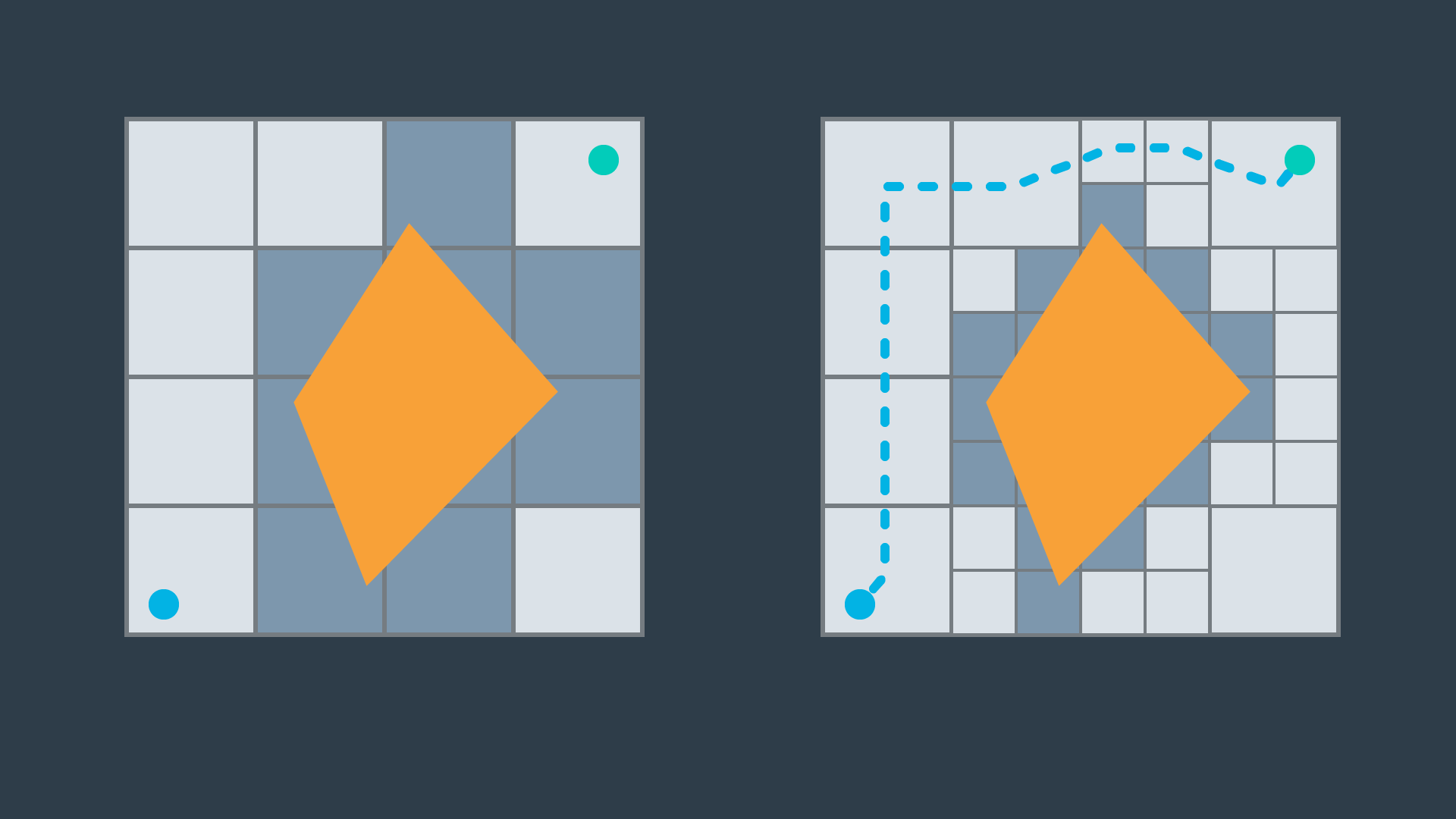
Decompose the configuration space into four cells, label cells free, mixed, or full.

Search for a sequence of free cells that connect the start node to the goal node.

if (sequence exists):
    Return path

else
    Further decompose the mixed cells

The three dimensional equivalent of quadtrees are octrees. The method of discretizing a space with any number of dimensions follows the same procedure as the algorithm described above, but expanded to accommodate the additional dimensions. 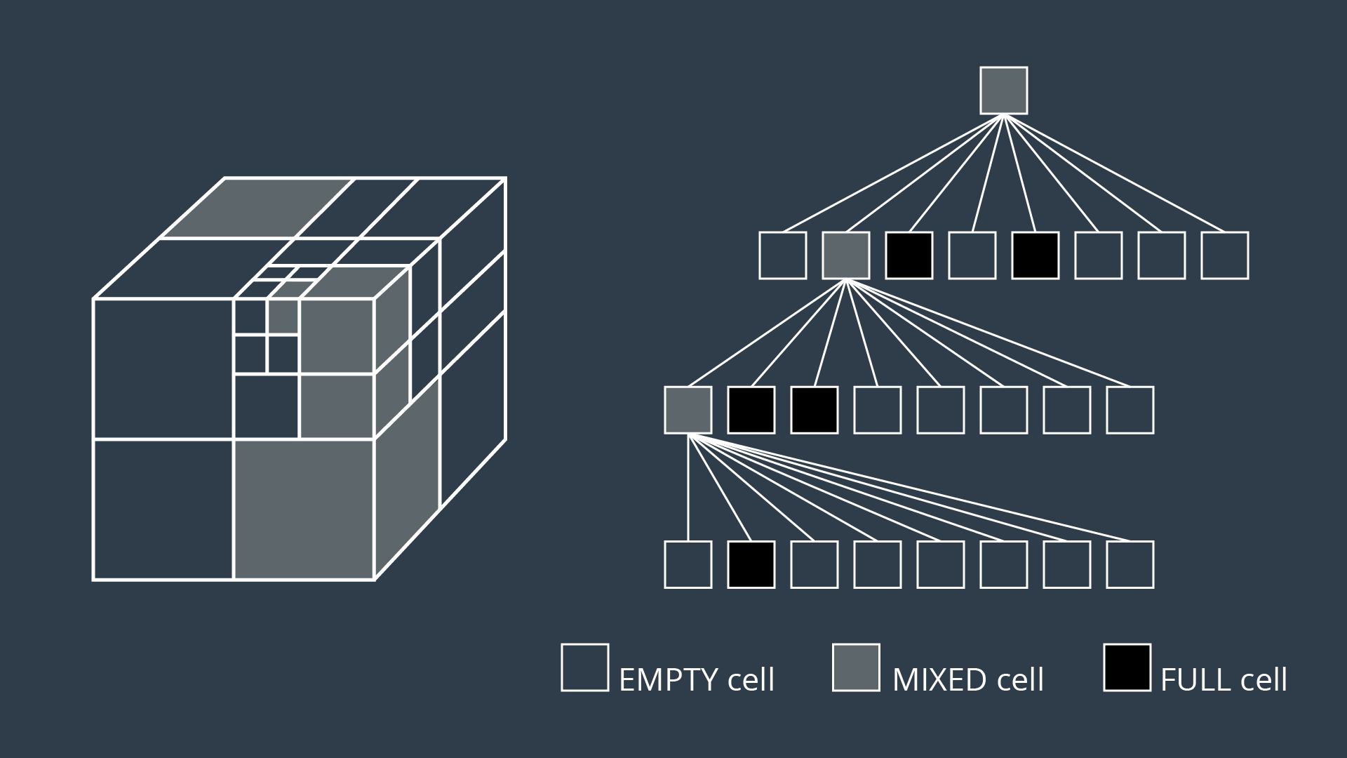Although exact cell decomposition is a more elegant method, it is much more computationally expensive than approximate cell decomposition for non-trivial environments. For this reason, approximate cell decomposition is commonly used in practice.

With enough computation, approximate cell decomposition approaches completeness. However, it is not optimal - the resultant path depends on how cells are decomposed. Approximate cell decomposition finds the obvious solution quickly. It is possible that the optimal path squeezes through a minuscule opening between obstacles, but the resultant path takes a much longer route through wide open spaces - one that the recursively-decomposing algorithms would find first.

Approximate cell decomposition is functional, but like all discrete/combinatorial path planning methods - it starts to be computationally intractable for use with high-dimensional environments.

Potential Field

Unlike the methods discussed thus far that discretize the continuous space into a connected graph, the potential field method performs a different type of discretization.

To accomplish its task, the potential field method generates two functions - one that attracts the robot to the goal and one that repels the robot away from obstacles. The two functions can be summed to create a discretized representation. By applying an optimization algorithm such as gradient descent, a robot can move toward the goal configuration while steering around obstacles.

Attractive Potential Field

The attractive potential field is a function with the global minimum at the goal configuration. If a robot is placed at any point and required to follow the direction of steepest descent, it will end up at the goal configuration. This function does not need to be complicated, a simple quadratic function can achieve all of the requirements discussed above.

$f_{att} (x) = \nu_{att} (||x-x_{goal}||)^{2}$

where x represents the robot's current position, and $x_{goal}$ the goal position. $/nu$ is a scaling factor.

A fragment of the attractive potential field:

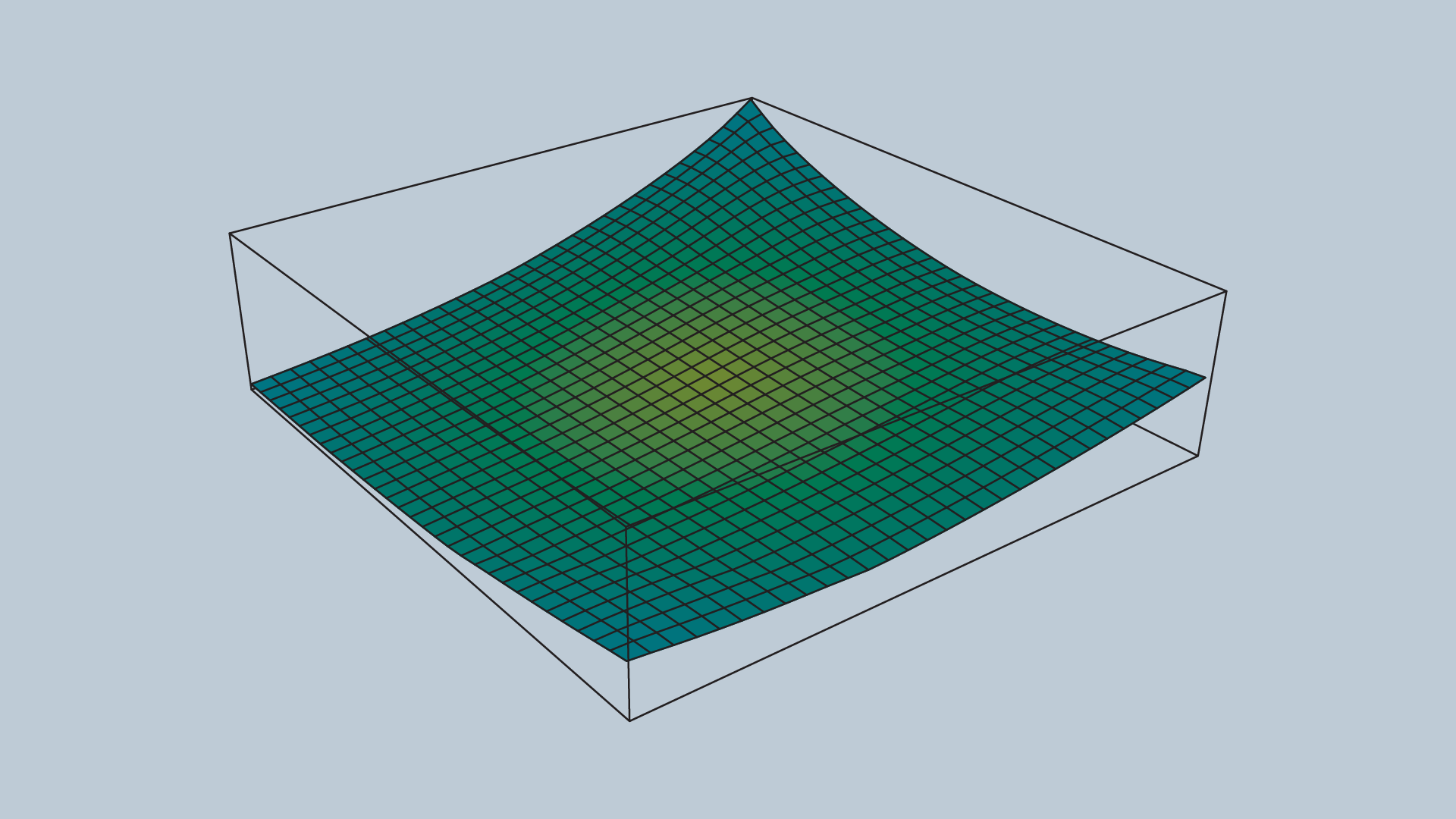
Repulsive Potential Field

The repulsive potential field is a function that is equal to zero in free space, and grows to a large value near obstacles. One way to create such a potential field.

$$\nu_{rep} (\frac{1}{\rho(x)} - \frac{1}{\rho_{0}})^{2} ~~~~ ~~~~ ~~~~ ~~~~ ~~~~ ~~~~ ~~~~ if \rho \leq \rho_{0}$$ $~~~~ ~~~~ ~~~~ ~~~~ ~~~~ ~~~~ ~~~~ ~~~~ ~~~~ ~~~~ f_{rep} ~~~~ ~~~~ ~~~~ = $

$$ 0 ~~~~~~~~~~~~~~~~~~~~~~~~~~~~~~~~~ if \rho > \rho_{0}$$

• The function $\rho (x)$ returns the distance from the robot to its nearest obstacle.
• $\rho_{0}$ is a scaling parameter that defines the reach of an obstacle's repulsiveness.
• $\nu$ is a scaling parameter.

An image of a repulsive potential field for an arbitrary configuration space

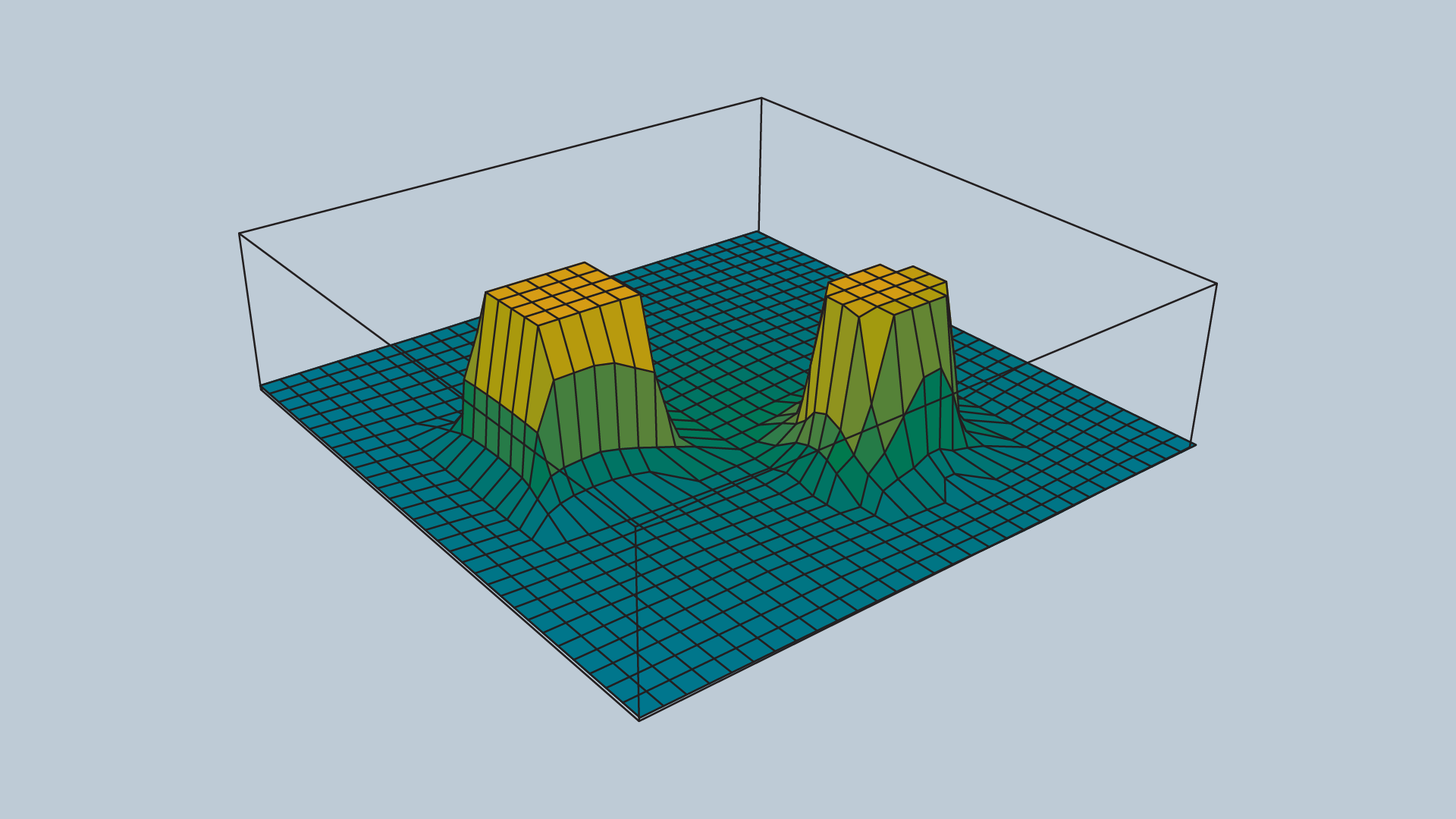
The value $\rho_{0}$ controls how far from an obstacle the potential field will be non-zero, and how steep the area surrounding an obstacle will be.

Potential Field Sum

The attractive and repulsive functions are summed to produce the potential field that is used to guide the robot from anywhere in the space to the goal. 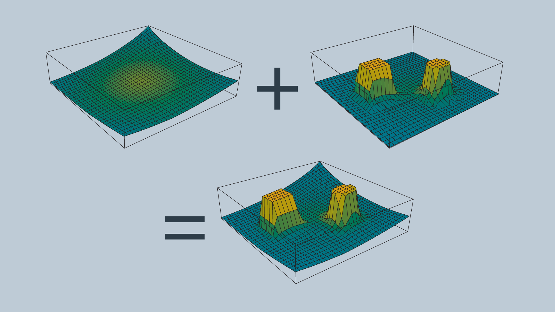The gradient of the function dictates which direction the robot should move, and the speed can be set to be constant or scaled in relation to the distance between the robot and the goal.

Graph Search

Graph Search is used to find finite sequence of discrete action to connect a start state to a goal state.

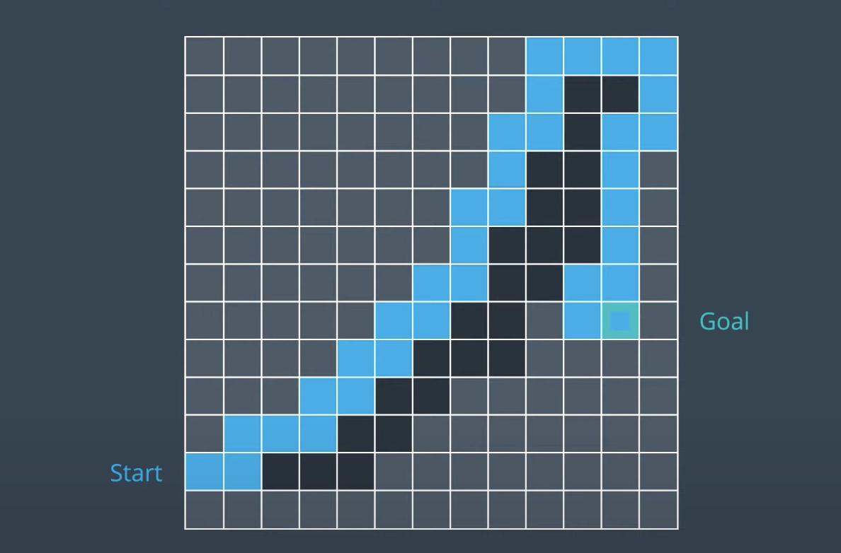
Types of Search Algorithm:

• Uniformed : Search blindly which are not provided with any information about the whereabouts of the goal. Breadth-First Search, Depth-First Search, Uniform Cost Search
• Informed : Can guid the search algorithm to make more intelligeent decisions which are provided with information pertaining to the location of the goal. A* search

Breadth-First Search (BFS)

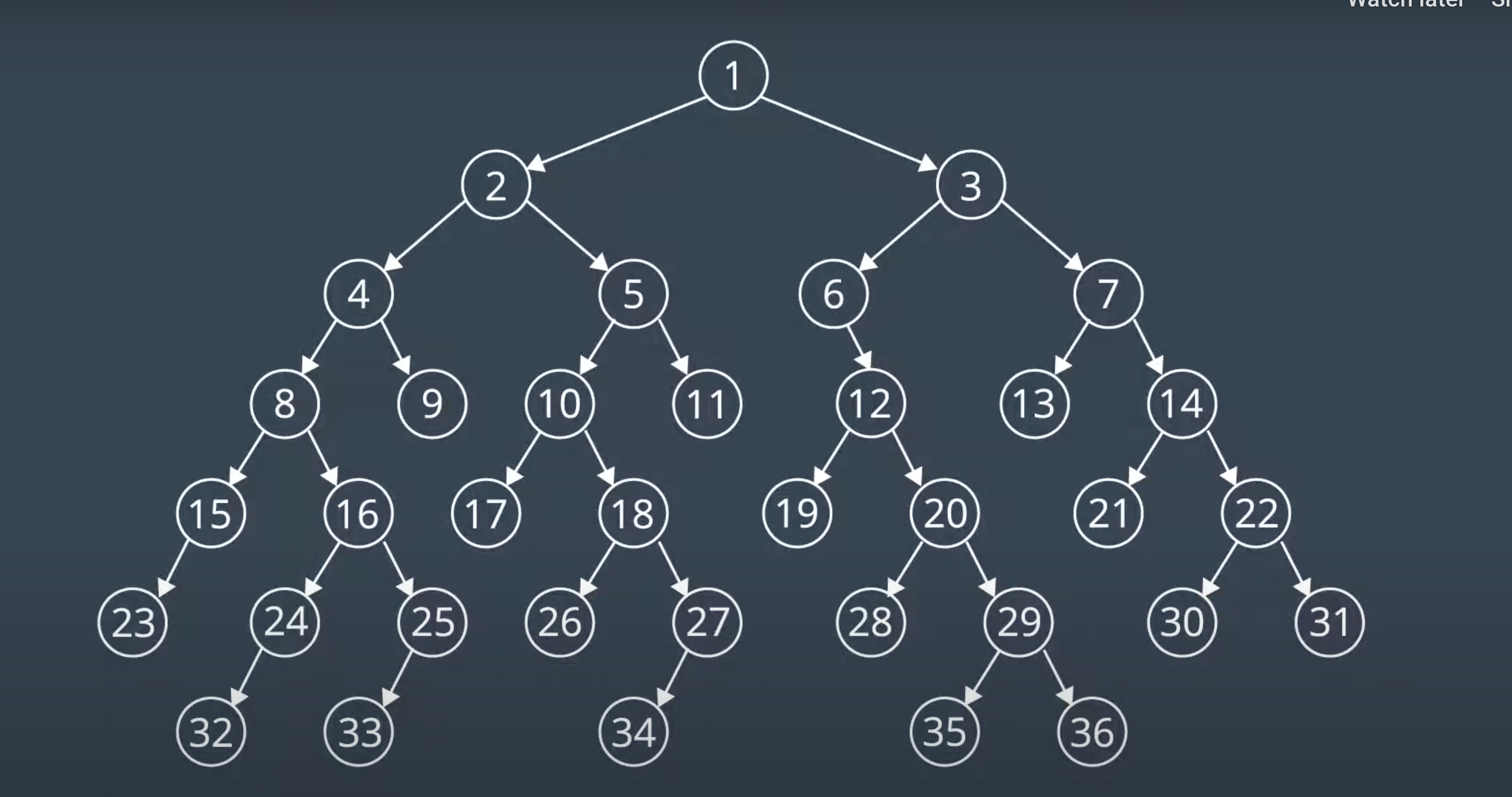Breadth-First Search is the data structure underlying the frontier is a queue. In a queue, the first element to enteer will be the first to exit. Add child nodes of the first node that will be added to frontier. BFS is still complete and optimal since it will always find goal soluttion. It is optimal because it will always find tthe shorteest solution since it explorees the shortest routes firs. It is optimal because it expands the shallowest unexplored node with every step. However BFS is limited to graphs wheere all step costs are equal. It also might take the algorithm a long time to find the solution. Therefore, algorithm is not efficient. 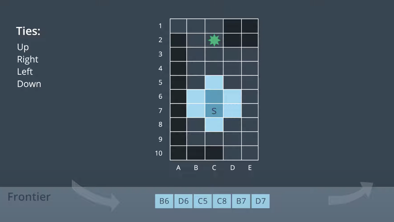Lab Path Planning

Depth-First Search (DFS)

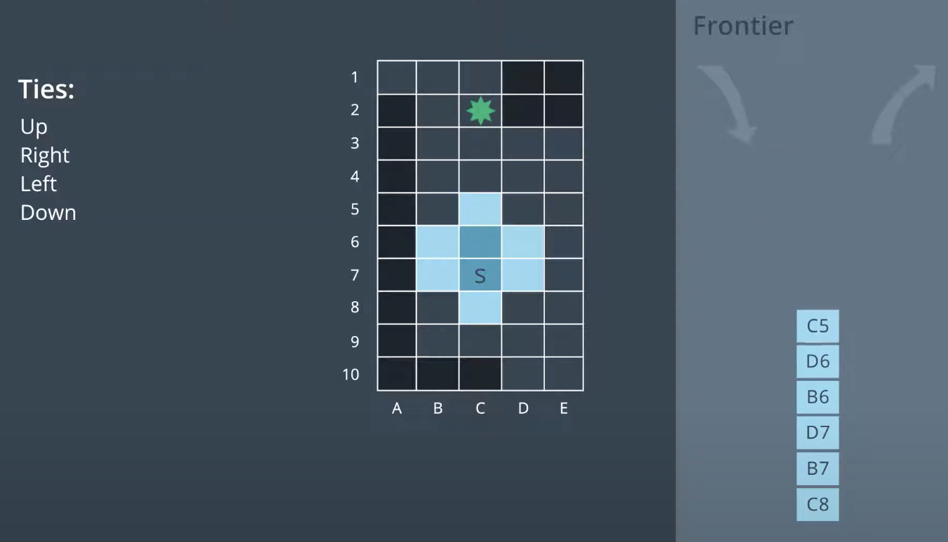
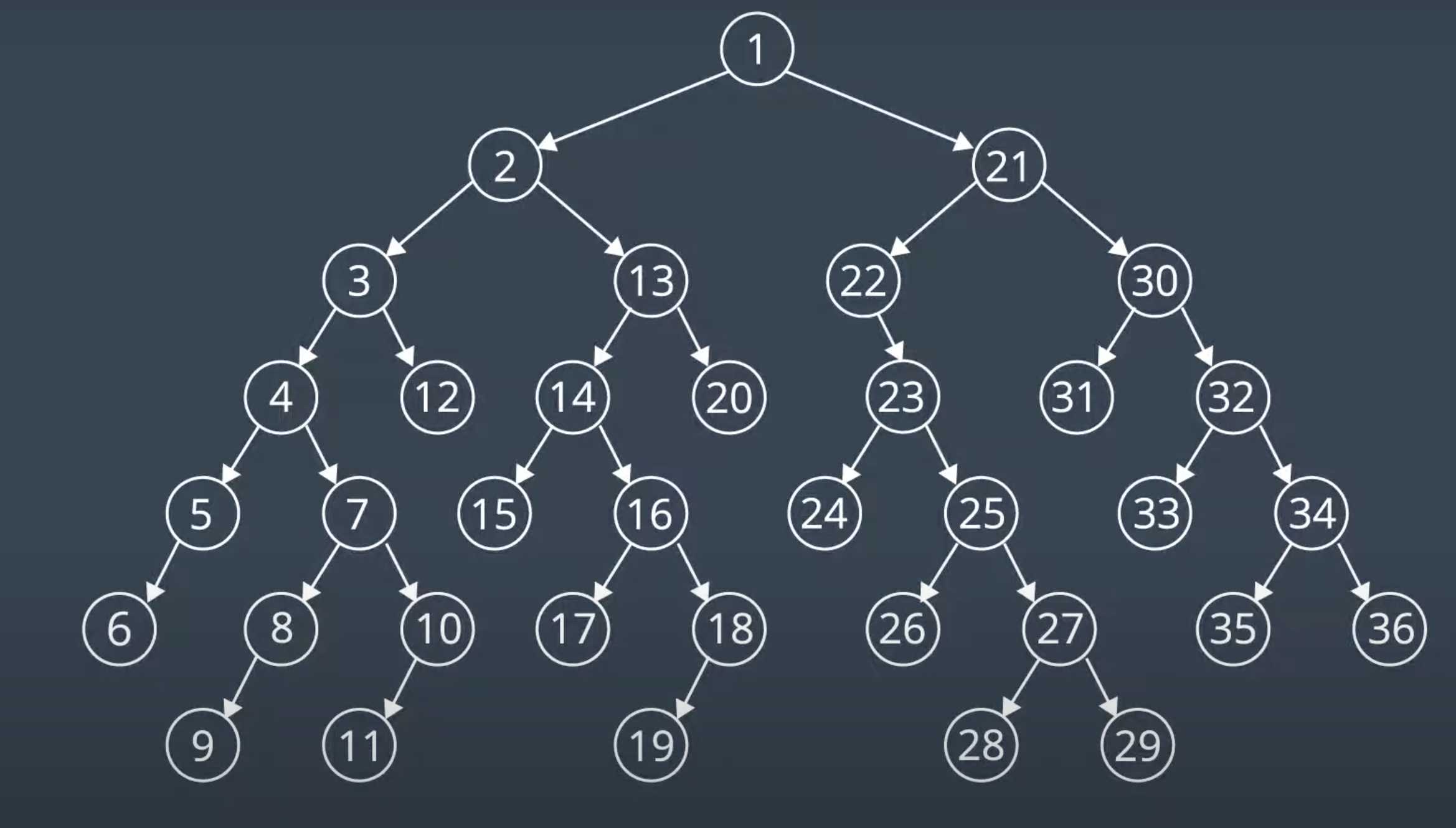Depth-First Search expand newly visited nodes first. The data structrue undrlying the frontier will be stack. DFS is exploring deep on the upwards direction. DFS is neither complete, nor optimal, nor efficient.

Uniform Cost Search

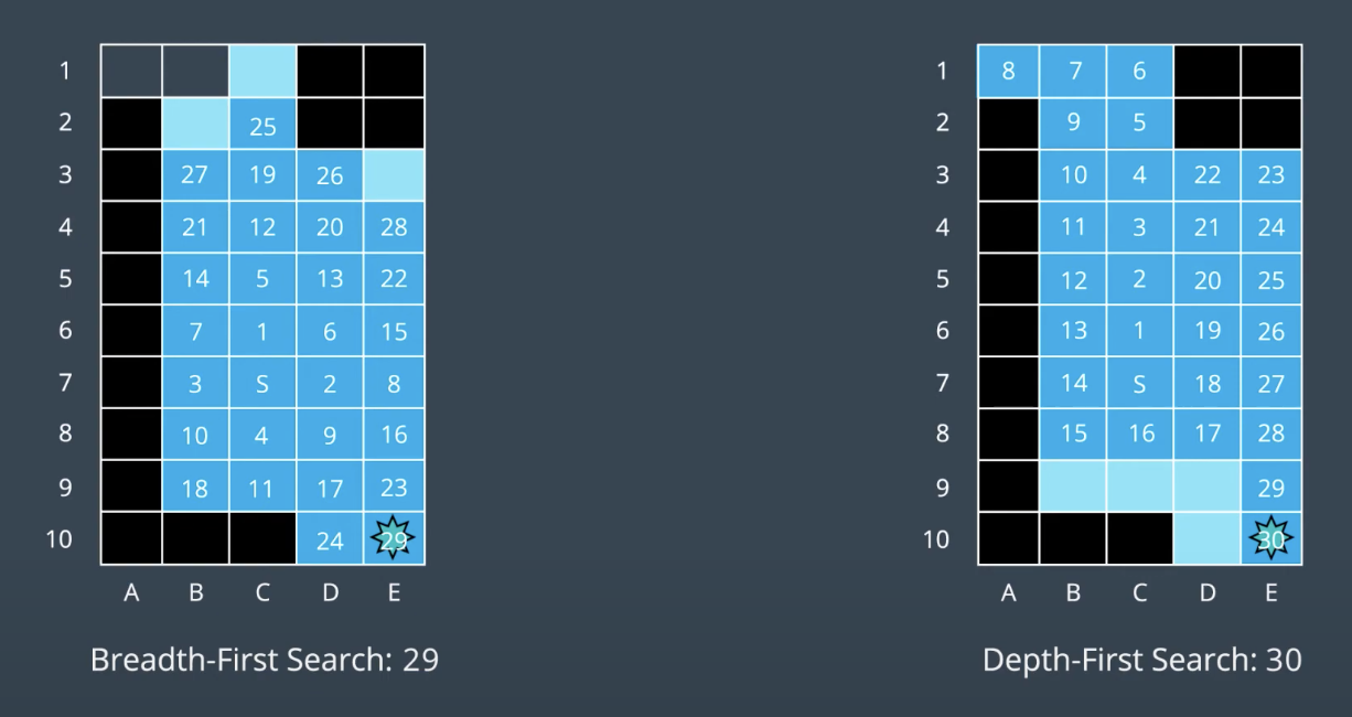As shown in BFS and DFS are not too efficient. Uniform Cost Search builds upon BfS to be able to search graphs with differing eedge costs. Uniform Cost Search is optimal because it expands nodes in order of increasing path cost. 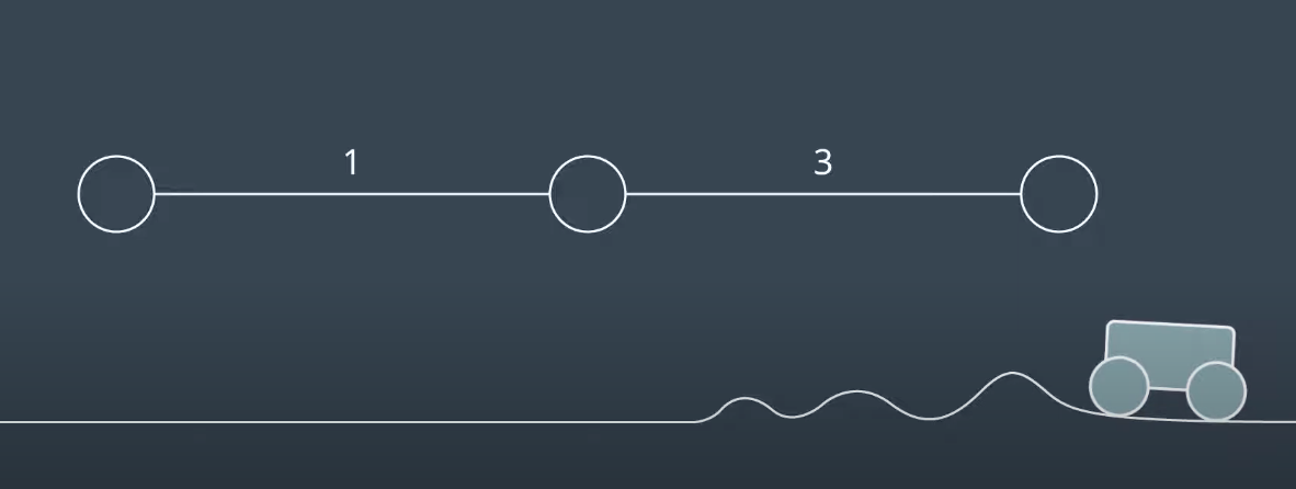As shown above higher cost to the edge is consider delay. The Uniform Cost Search splores the node of the frontier starting with the node that has the lowest path cost. Path Cost refers to the sum of all edge costs leading from the start to the node. 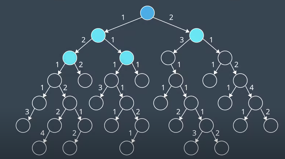As shown above the first child nodes of path costs are 1<2 which start to explore lowst costs (left node).

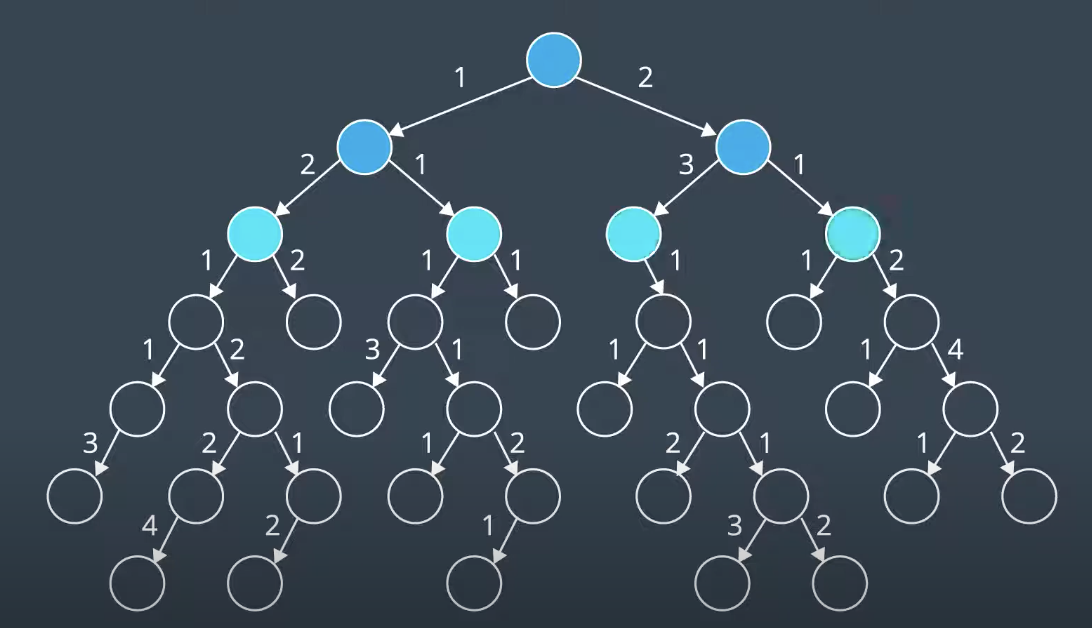
Uniform Cost search explore nodes with lowest path costs first. To accommodate this, it use a priority queue that is a queue that is organized by the path cost.

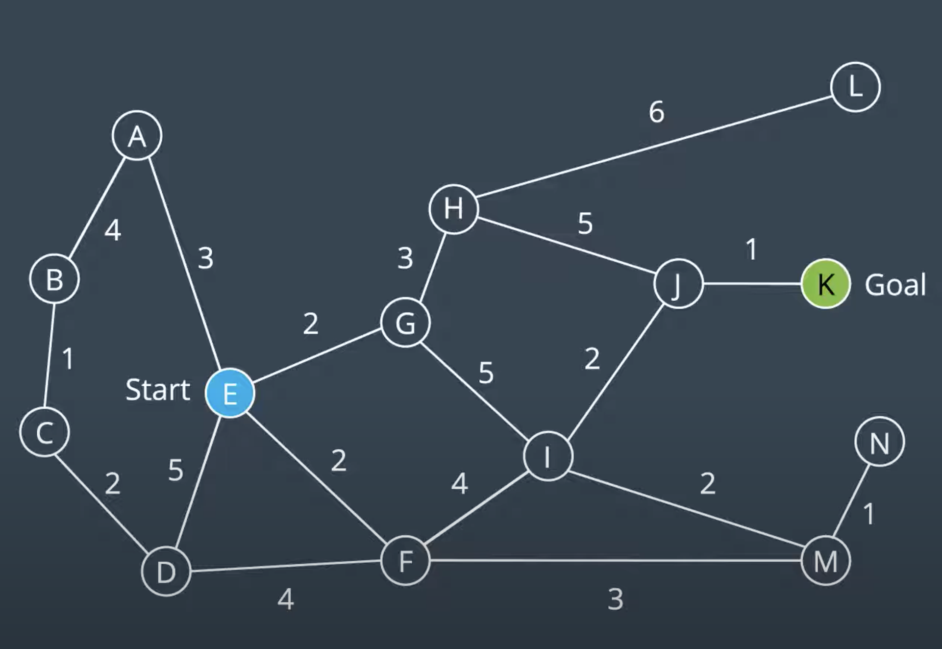
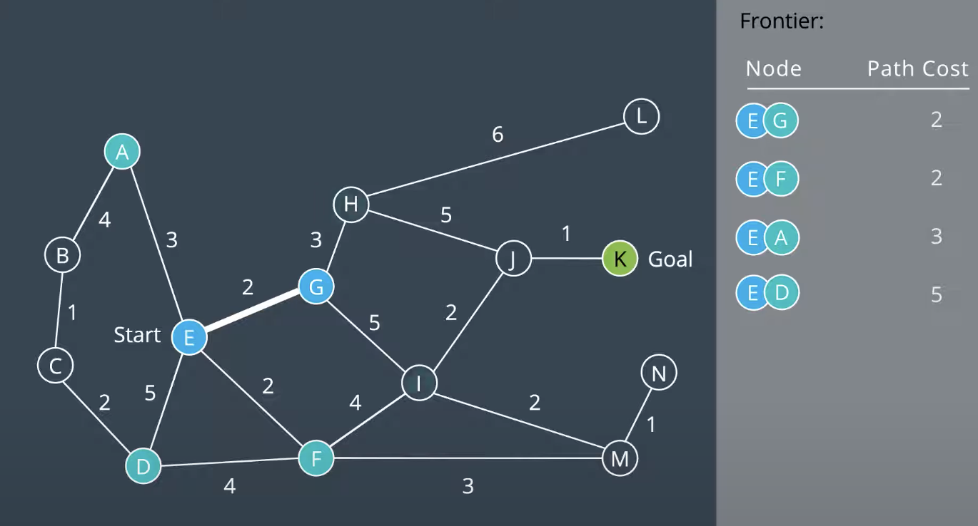
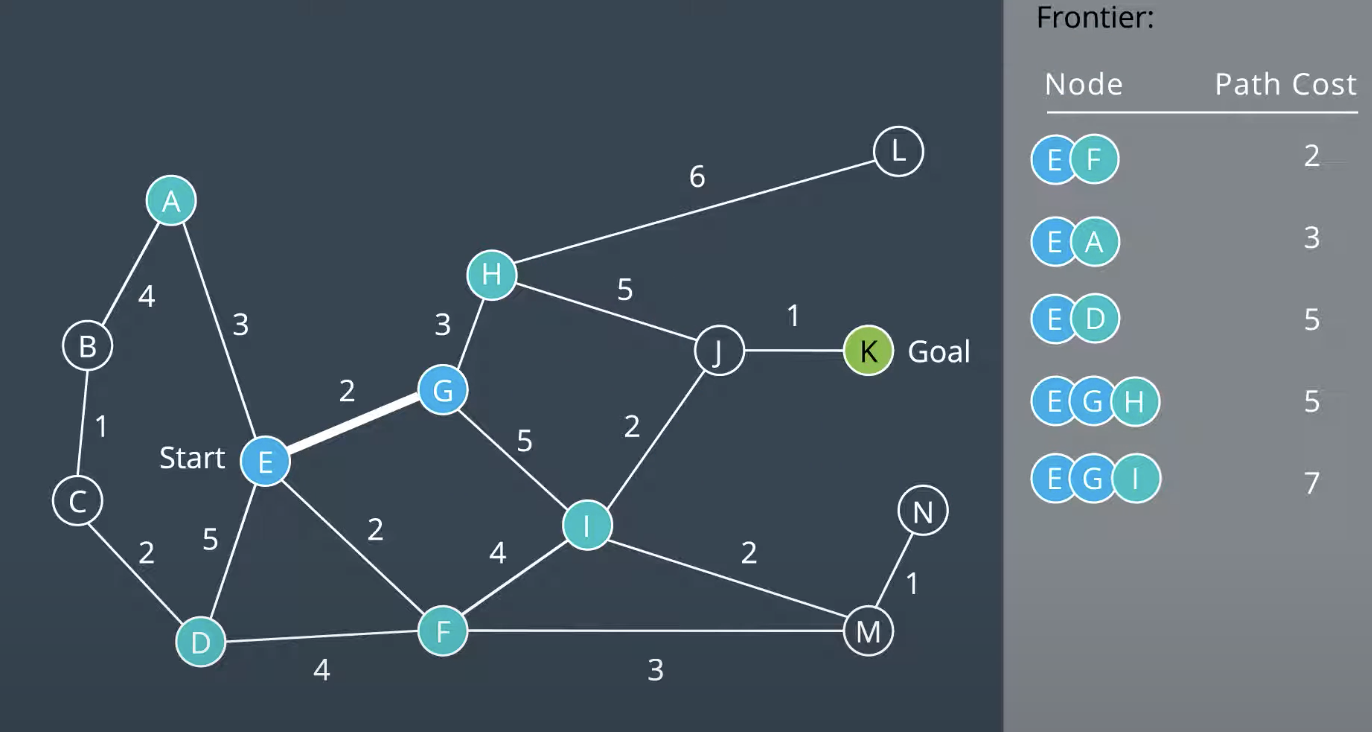
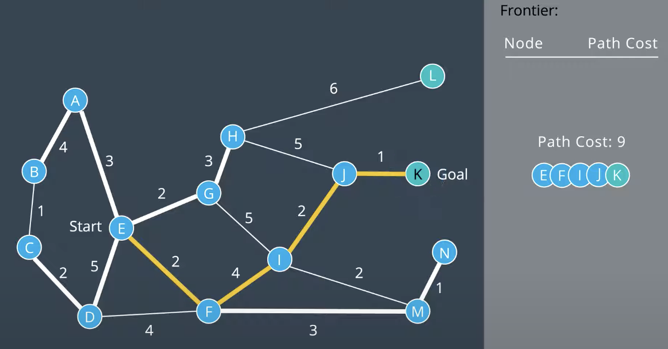
Uniform Cost Search is complete if every step cost is greater than some value, otherwise it can get stuck in infinitee loops. And it is also optimal.

**** A* Search A* Search is an informed search. This means that it takes into account information about the goal's location as it goes aboout its search. It uses a heuristic function.

h(n) = distance to goal 
g(n) = path cost
f(n) = g(n) + h(n)

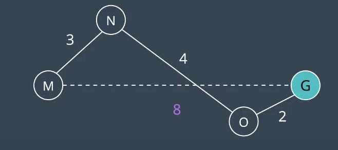
It represents the distance from a node to the goal. It is estimation of the distance as the only way to know the true distance would be to traverse the graph. 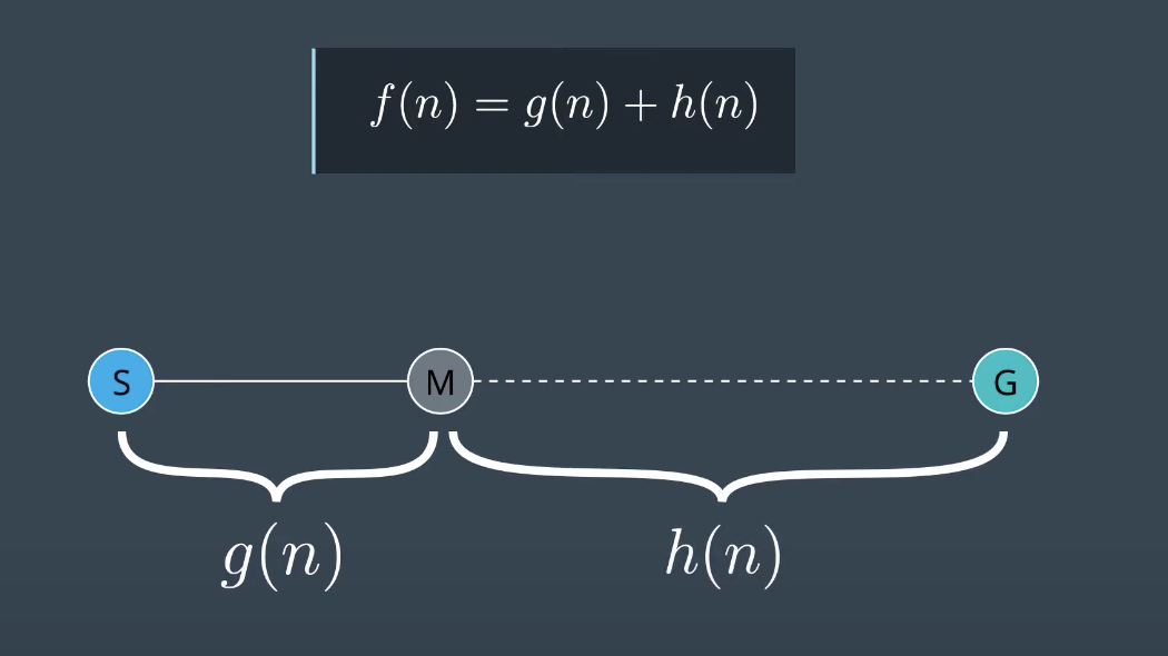Minimizing g(n) favors shorter paths and minimizing h(n) favors paths in the direction of the goal. A* searches for the shortest path in the direction of the goal. For valid heuristic, h(x) would be the Euclidean distance from a node to the goal. Nodes close to the goal have a low heuristic value, and nodes further away from the goal have a higher heeuristic value. As shown below, The goal itself has a heuristic of zero. In A* use Priority Queue as the data structure underlying the frontier. Unlike UCS, A* search is directed towards the goal. The nodes on the left hand side of the graaph have not been explored. This instance where nodes' path and f(n) value aree updated based on h(n).

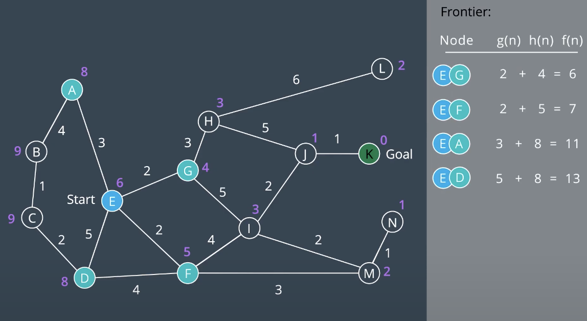
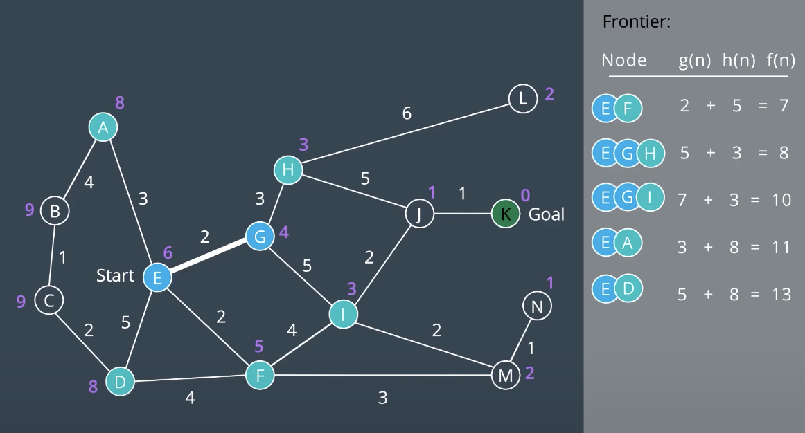
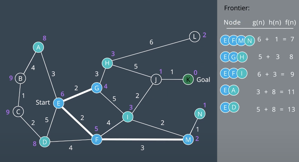
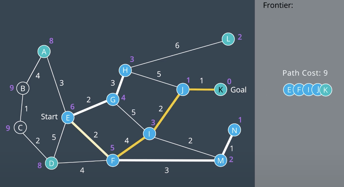A heuristic function provides the robot with knowledge about the environment, guiding it in the direction of the goal. A* uses tthe sum of the path cost and the heuristic function to determine which nodes to explore next. Choosing an appropriate heuristic function(Euclidean distance, Manhattan distance, etc) is importnat. the order in which nodes are explored will change from one heuristic to another. However, A* search algorithm isn’t guaranteed to be optimal.

A* search will find the optimal path if* the following conditions are met:

• Every edge must have a cost greater than some value, ϵ, otherwise, the search can get stuck in infinite loops and the search would not be complete.
• The heuristic function must be consistent. This means that it must obey the triangle inequality theorem. That is, for three neighbouring points ( $x_{1}, x_{2}, x_{3}$ ), tthe heuristic value for $x_{1}$ to $x_{3}$ must be less than the sum of the heuristic values for $x_{1}$ to $x_{2}$ and $x_{2}$ to $x_{3}$.
• The heuristic function must be admissible. This means that h(n) must always be less than or equal to the true cost of reaching the goal from every node. In other words, h(n) must never overestimate the true path cost.

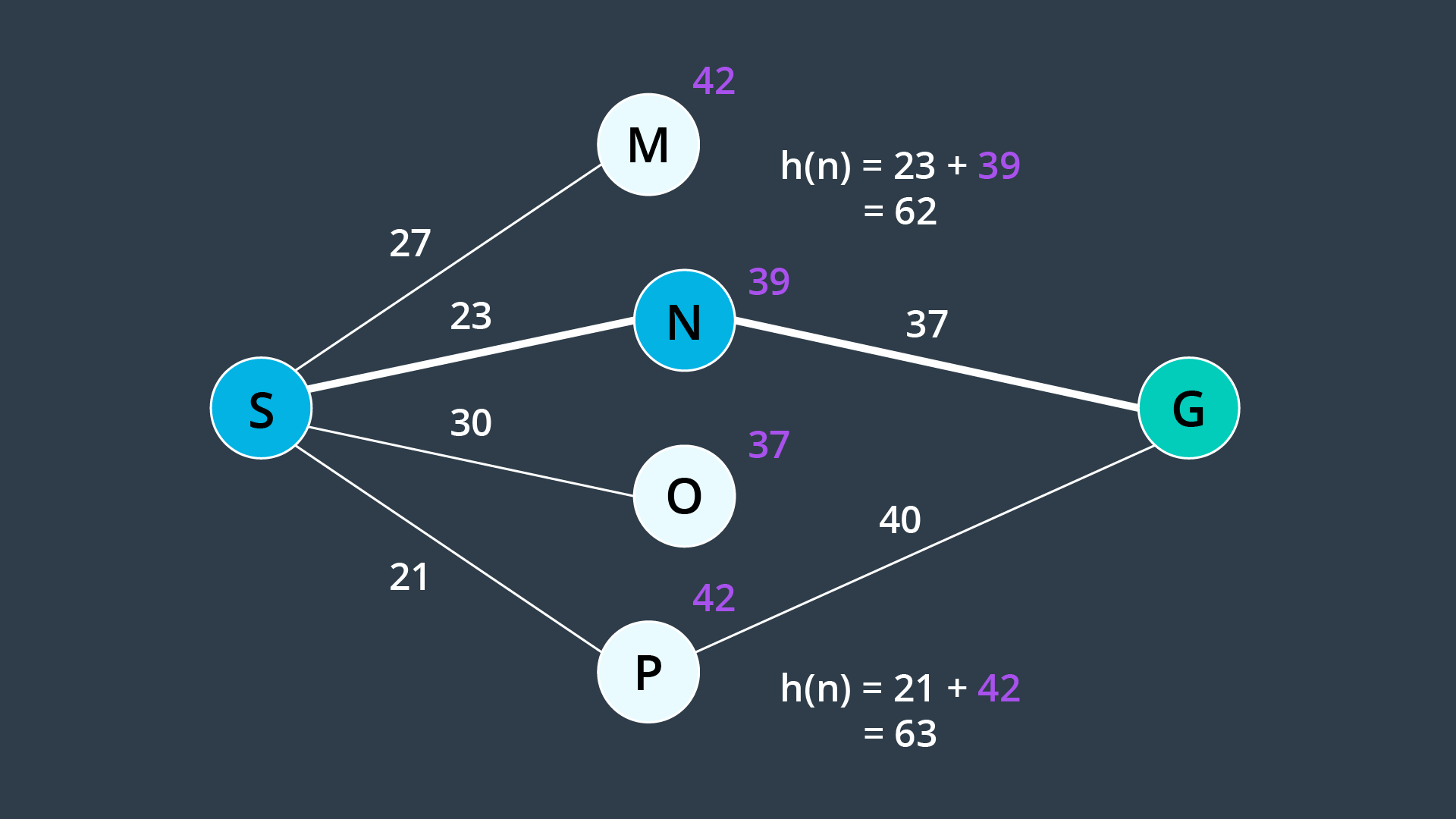
As shown above, to understand where the admissibility clause comes from. Suppose you have two paths to a goal where one is optimal (the highlighted path), and one is not (the lower path). Both heuristics overestimate the path cost. From the start, you have four nodes on the frontier, but Node N would be expanded first because its h(n) is the lowest - it is equal to 62. From there, the goal node is added to the frontier - with a cost of 23 + 37 = 60. This node looks more promising than Node P, whose h(n) is equal to 63. In such a case, A* finds a path to the goal which is not optimal. If the heuristics never overestimated the true cost, this situation would not occur because Node P would look more promising than Node N and be explored first.

Admissibility is a requirement for A* to be optimal. For this reason, common heuristics include the Euclidean distance from a node to the goal or in some applications the Manhattan distance. When comparing two different types of values - for instance, if the path cost is measured in hours, but the heuristic function is estimating distance - then you would need to determine a scaling parameter to be able to sum the two in a useful manner.

Lab Path Planning

Bidirectional Search

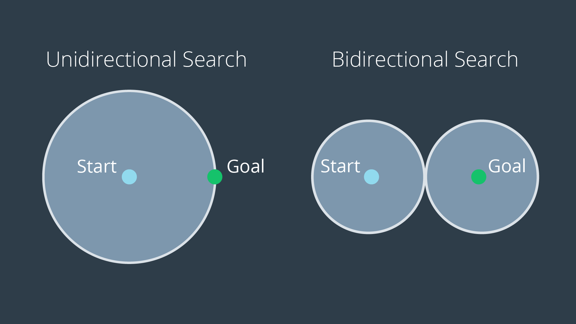
One way to improve a search’s efficiency is to conduct two searches simultaneously - one rooted at the start node, and another at the goal node. Once the two searches meet, a path exists between the start node and the goal node.

The advantage with this approach is that the number of nodes that need to be expanded as part of the search is decreased. As you can see in the image below, the volume swept out by a unidirectional search is noticeably greater than the volume swept out by a bidirectional search for the same problem.

Path Proximity to Obstacles

Another concern with the search of discretized spaces includes the proximity of the final path to obstacles or other hazards. When discretizing a space with methods such as cell decomposition, empty cells are not differentiated from one another. The optimal path will often lead the robot very close to obstacles. In certain scenarios this can be quite problematic, as it will increase the chance of collisions due to the uncertainty of robot localization. The optimal path may not be the best path. To avoid this, a map can be ‘smoothed’ prior to applying a search to it, marking cells near obstacles with a higher cost than free cells. Then the path found by A* search may pass by obstacles with some additional clearance.

Paths Aligned to Grid

Another concern with discretized spaces is that the resultant path will follow the discrete cells. When a robot goes to execute the path in the real world, it may seem funny to see a robot zig-zag its way across a room instead of driving down the room’s diagonal. In such a scenario, a path that is optimal in the discretized space may be suboptimal in the real world. Some careful path smoothing, with attention paid to the location of obstacles, can fix this problem.

Sample-Based Planning

Sample-based path planning probes the workspace to incrementally construct a graph. Instead of discretizing every segment of the workspace, sample-based planning takes a number of samples and uses them to build a discrete representation of the workspace. The resultant graph is not as precise as one created using discrete planning, but it is much quicker to construct because of the relatively small number of samples used. A path generated using sample-based planning may not be the best path, but in certain applications - it’s better to generate a feasible path quickly than to wait hours or even days to generate the optimal path.

Why Sample-Based Planning?

Discrete planning for higher dimensional problems are incredibly hard to discretize such a large space. The complexity of the path planning problem increases exponentially with the number of dimensions in the C-space.

Increased Dimensionality

For a 2-dimensional 8-connected space, every node has 8 successors (8-connected means that from every cell you can move laterally or diagonally). Imagine a 3-dimensional 8-connected space, how many successors would every node have? 26. As the dimension of the C-space grows, the number of successors that every cell has increases substantially. In fact, for an n-dimensional space, it is equal to $3^n -1$. The robotic arm that you worked with in the pick-and-place project - that was a 6-DOF arm. If multiple 6-DOF arms work in a common space, the computation required to perform path planning to avoid collisions increases substantially. Then, think about the complexity of planning for humanoid robots such as the one depicted below. Such problems may take intolerably long to solve using the combinatorial approach.

Constrained Dynamics

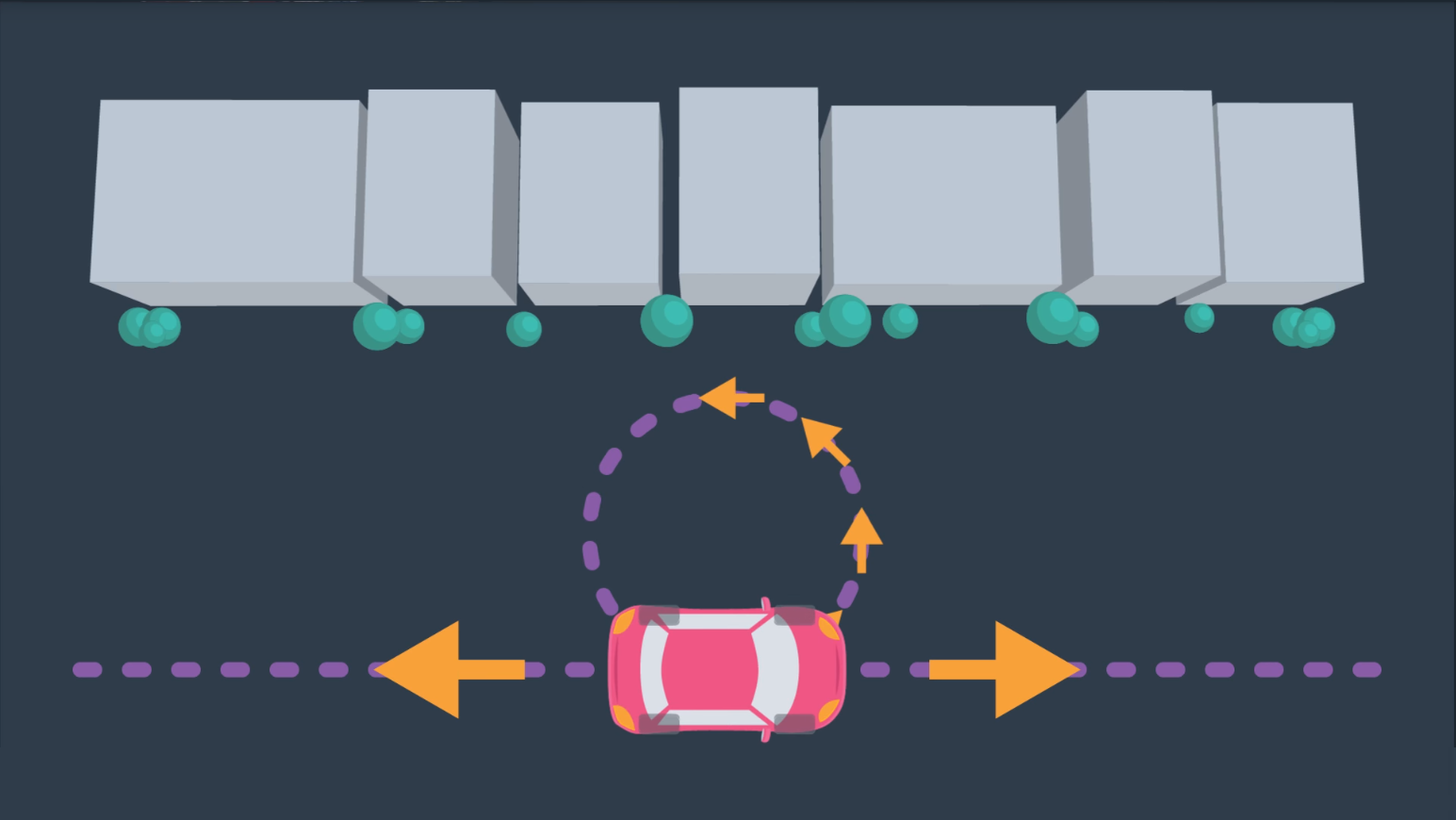
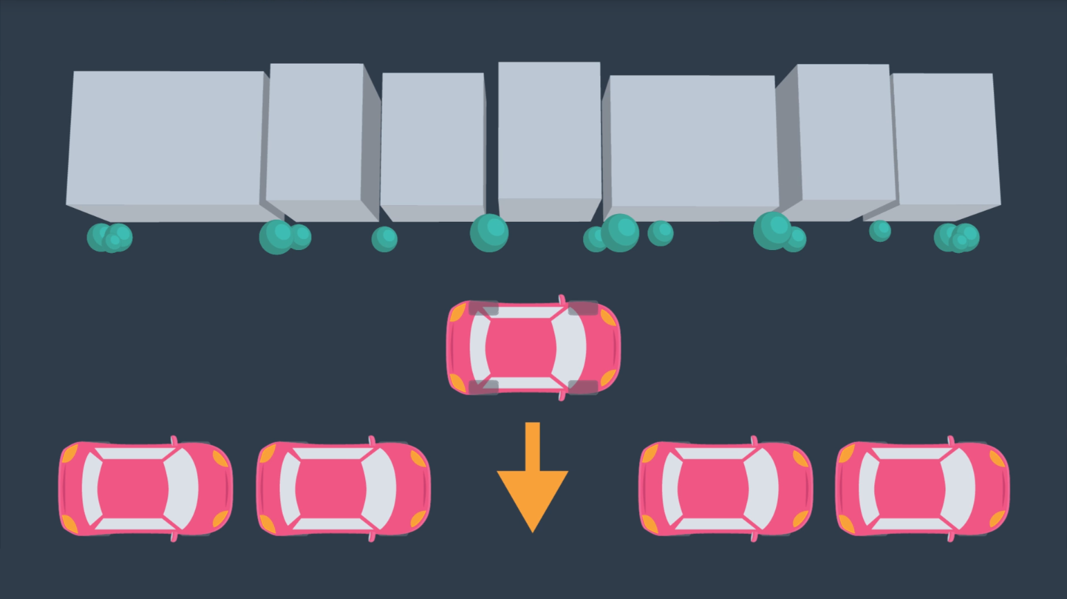
Aside from robots with many degrees of freedom and multi-robot systems, another computational difficulty involves working with robots that have constrained dynamics. For instance, a car is limited in its motion - it can move forward and backward, and it can turn with a limited turning radius as below. However, the car is not able to move laterally as depicted in the following image, struggle to parallel park. In the case of the car, more complex motion dynamics must be considered when path planning - including the derivatives of the state variables such as velocity. For example, a car's safe turning radius is dependent on it's velocity.

Robotic systems can be classified into two different categories:

• Holonomic systems can be defined as systems where every constraint depends exclusively on the current pose and time, and not on any derivatives with respect to time.

• Nonholonomic systems, on the other hand, are dependent on derivatives. Path planning for nonholonomic systems is more difficult due to the added constraints.

Weakening Requirements

Combinatorial path planning algorithms are too inefficient to apply in high-dimensional environments, which means that some practical compromise is required to solve the problem! Instead of looking for a path planning algorithm that is both complete and optimal, what if the requirements of the algorithm were weakened?

Instead of aspiring to use an algorithm that is complete, the requirement can be weakened to use an algorithm that is probabilistically complete. A probabilistically complete algorithm is one who’s probability of finding a path, if one exists, increases to 1 as time goes to infinity.

Similarly, the requirement of an optimal path can be weakened to that of a feasible path. A feasible path is one that obeys all environmental and robot constraints such as obstacles and motion constraints. For high-dimensional problems with long computational times, it may take unacceptably long to find the optimal path, whereas a feasible path can be found with relative ease. Finding a feasible path proves that a path from start to goal exists, and if needed, the path can be optimized locally to improve performance.

*Sample-based planning is probabilistically complete and looks for a feasible path instead of the optimal path.

Sample-Based Planning

Sample-based path planning differs from combinatorial path planning in that it does not try to systematically discretize the entire configuration space. Instead, it samples the configuration space randomly (or semi-randomly) to build up a representation of the space. The resultant graph is not as precise as one created using combinatorial planning, but it is much quicker to construct because of the relatively small number of samples used.

Such a method is probabilistically complete because as time passes and the number of samples approaches infinity, the probability of finding a path, if one exists, approaches 1.

Such an approach is very effective in high-dimensional spaces, however it does have some downfalls. Sampling a space uniformly is not likely to reach small or narrow areas, such as the passage depicted in the image below. Since the passage is the only way to move from start to goal, it is critical that a sufficient number of samples occupy the passage, or the algorithm will return ‘no solution found’ to a problem that clearly has a solution.

Different sample-based planning approaches exist, each with their own benefits and downfalls.

• Probabilistic Roadmap Method
• Rapidly Exploring Random Tree Method

Probabilistic Roadmap (PRM)

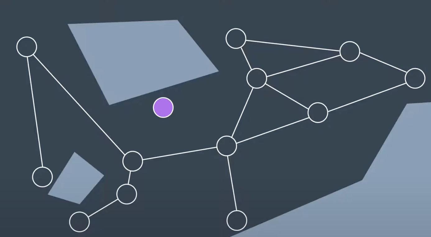
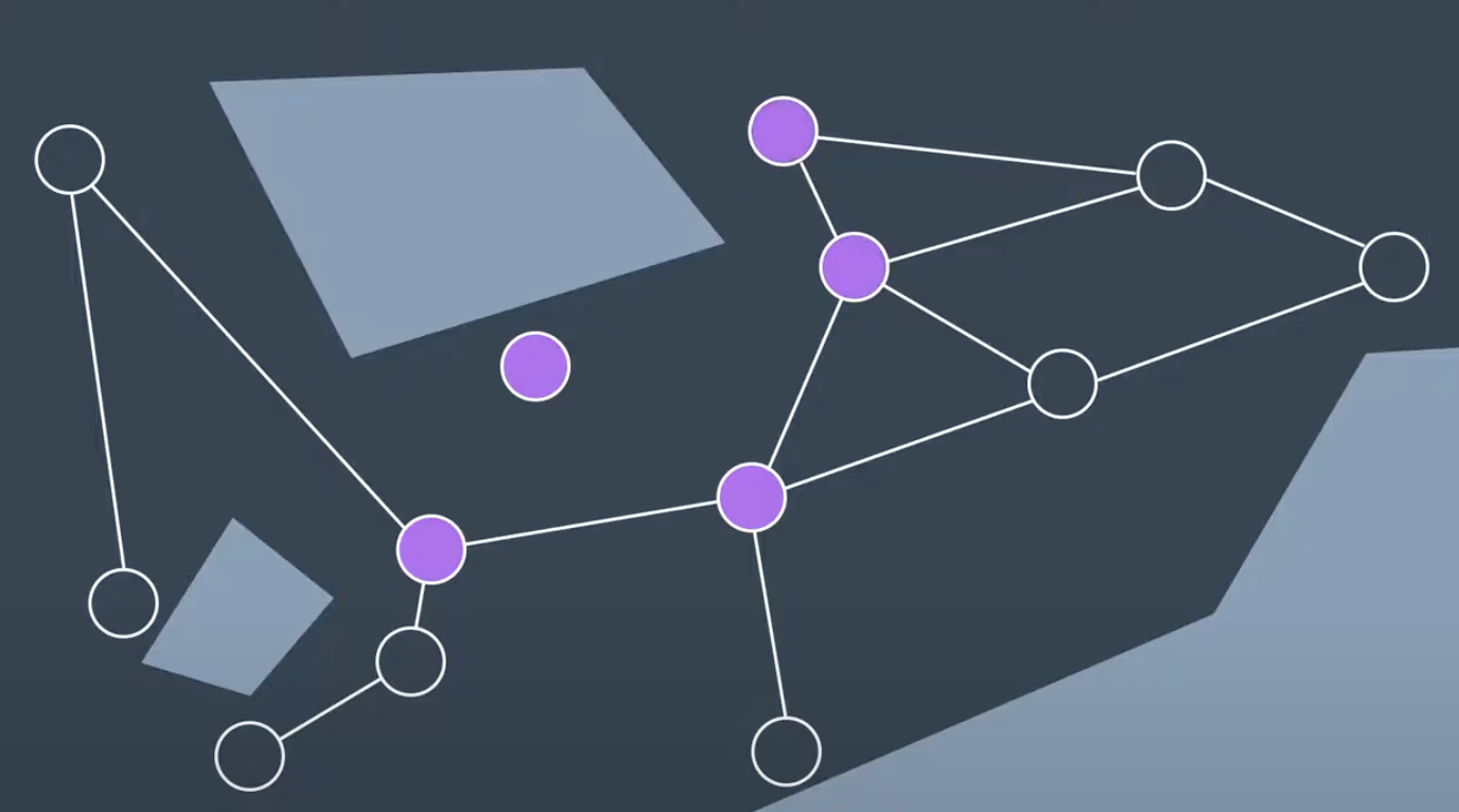
One common sample-based path planning method is called probablistic roadmap(PRM). PRM randomly samples the workspace, building up a graph to represent the free space. All the PRM require is a collision check function to test whether a randomly generated node lies in the freespace or is in collision with an obstacle.

The process of building up a graph is called the learning phase.

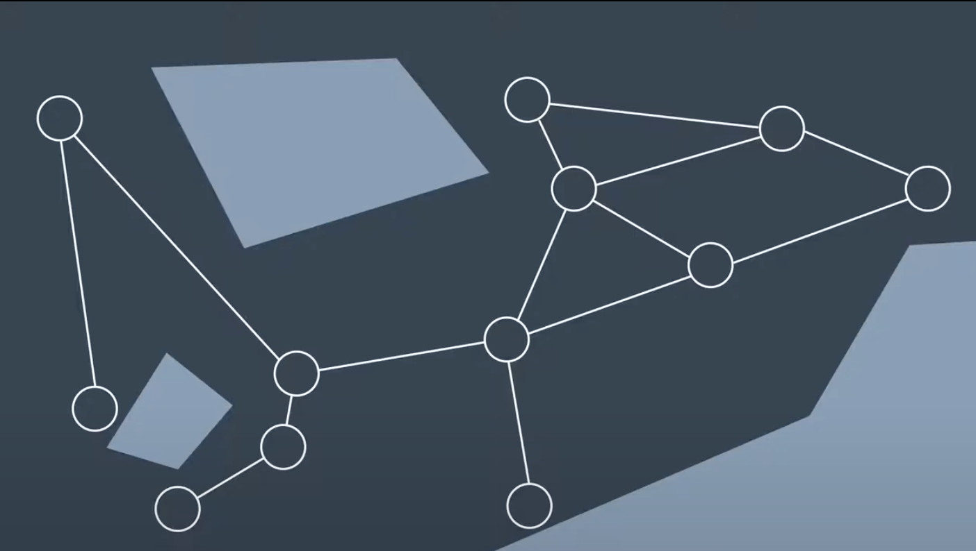
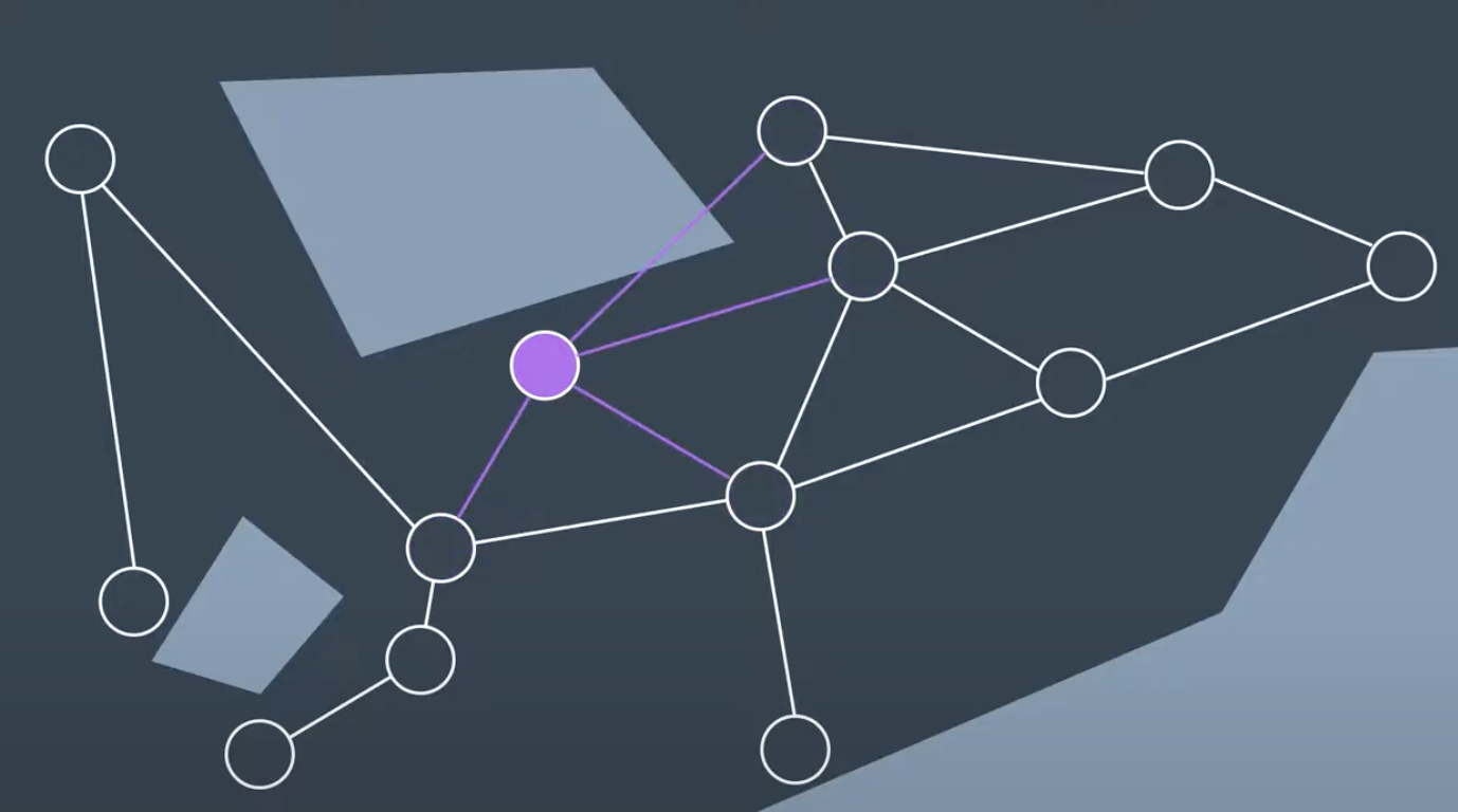
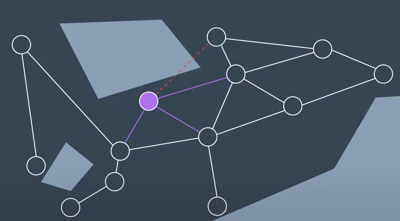
It does so by generating a new random configuratiion represented by a node in the graph and checking to see if it is in collision. If node is not in collision, then PRM will try to connectt the node to its neighbors.

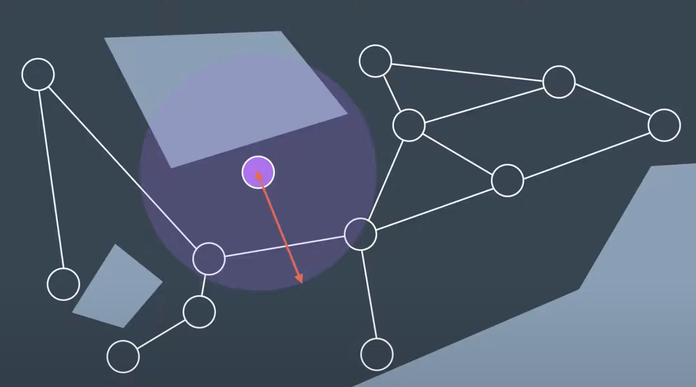
There are few different way to connect. PRM can look for any number of neighbors within a certain radius of the node or it could look for thee nodes K nearest neighbors. Once the neighbors have been selected, PRM will see if they can successfully create an edge of its neighbors.

As you see below, one edge is in collision with obstacle while other three are safe to add. This node has been added to the graph, and repeat for another randomly generated node.

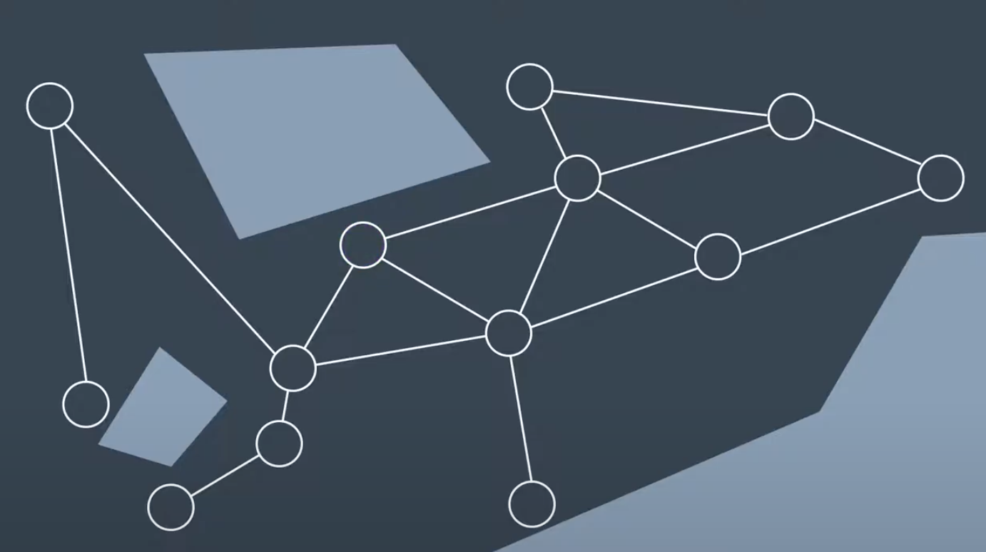
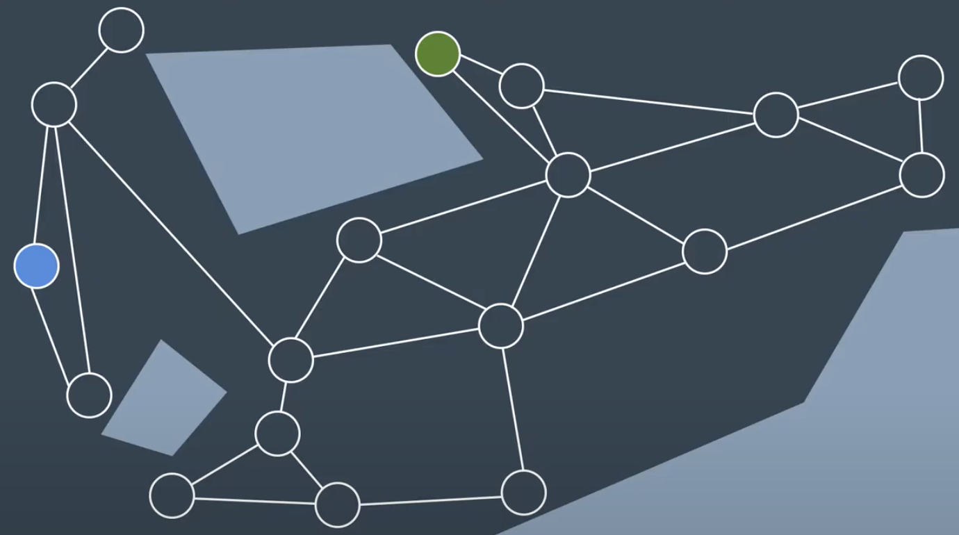
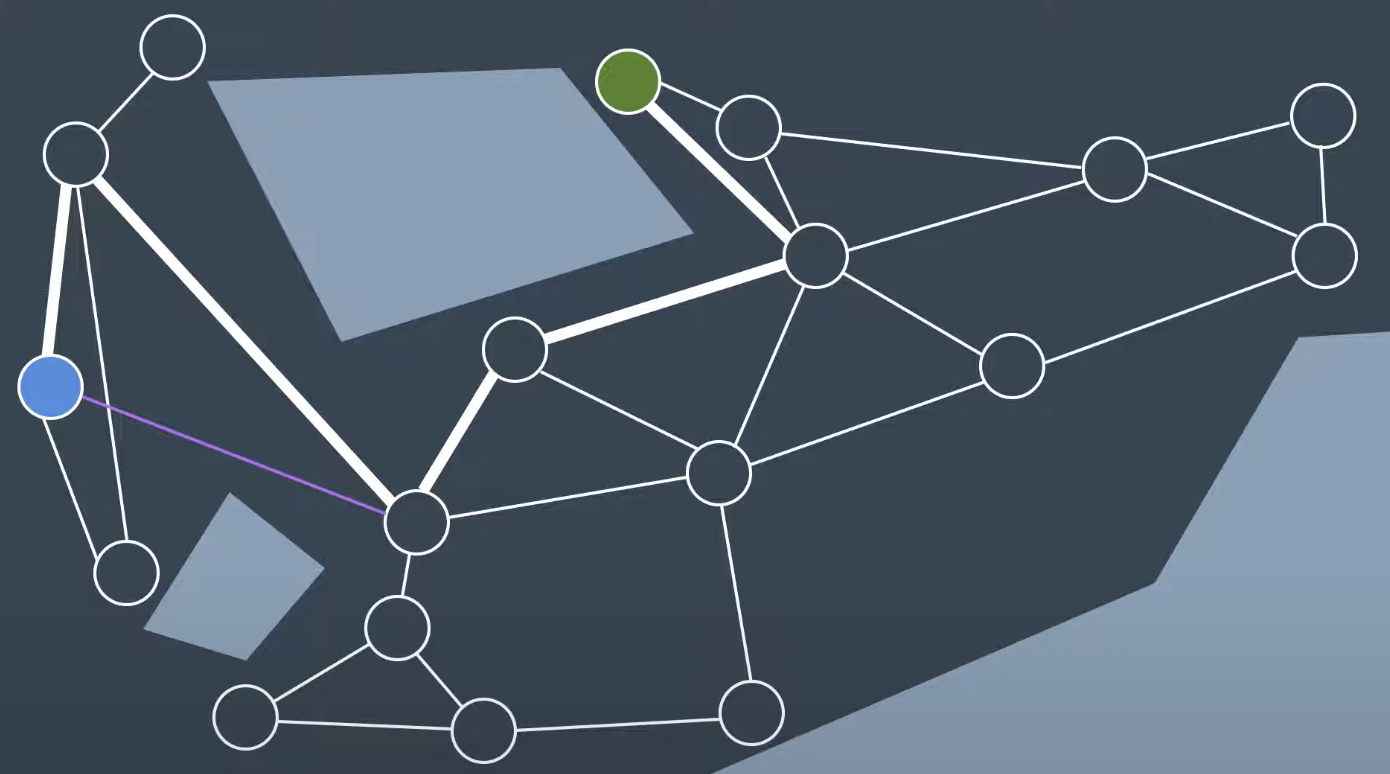
First, it must connect each of these start to the graph. PRM does so by looking for the nodes closest to the start and goal and using the local planner to try to build a connection.

When the learning phase is over, then PRM enters the queery phase where it uses the resulting graph to find a path from start to goal. If the process is successful then a search algorithm like A star search can be applied to find the path from start to goal.

Algorithm: Pseudocode for the PRM learning phase:

Initialize an empty graph
For n iterations:

   Generate a random configuration.
   If the configuration is collision free: 

      Add the configuration to the graph.
      Find the k-nearest neighbours of the configuration.
      For each of the k neighbours:

         Try to find a collision-free path between 
            the neighbour and original configuration. 
            If edge is collision-free: 
                Add it to the graph. 

After the learning phase, comes the query phase.

Setting Parameters

There are several parameters in the PRM algorithm that require tweaking to achieve success in a particular application.

• the number of iterations can be adjusted: the parameter controls between how detailed the resultant graph is and how long the computation takes. For path planning problems in wide-open spaces, additional detail is unlikely to significantly improve the resultant path. However, the additional computation is required in complicated environments with narrow passages between obstacles. Beware, setting an insufficient number of iterations can result in a ‘path not found’ if the samples do not adequately represent the space.

• Another decision that a robotics engineer would need to make is how to find neighbors for a randomly generated configuration. One option is to look for the k-nearest neighbors to a node. To do so efficiently, a k-d tree can be utilized - to break up the space into ‘bins’ with nodes, and then search the bins for the nearest nodes. Another option is to search for any nodes within a certain distance of the goal. Ultimately, knowledge of the environment and the solution requirements will drive this decision-making process.

• The choice for what type of local planner to use is another decision that needs to be made by the robotics engineer. The local planner demonstrated in the above is an example of a very simple planner. For most scenarios, a simple planner is preferred, as the process of checking an edge for collisions is repeated many times (k*n times, to be exact) and efficiency is key. However, more powerful planners may be required in certain problems. In such a case, the local planner could even be another PRM.

Probabilistically Complete

Sample-based path planning algorithms are probabilistically complete. As the number of iterations approaches infinity, the graph approaches completeness and the optimal path through the graph approaches the optimal path in reality.

Variants

Current algorith as shown above is vanilla version of PRM, but many other variations to it exist. A Comparative Study of Probabilistic Roadmap Planners

PRM is a Multi-Query Planner

The Learning Phase takes significantly longer to implement than the Query Phase, which only has to connect the start and goal nodes, and then search for a path. However, the graph created by the Learning Phase can be reused for many subsequent queries. For this reason, PRM is called a multi-query planner.

This is very beneficial in static or mildly-changing environments. However, some environments change so quickly that PRM’s multi-query property cannot be exploited. In such situations, PRM’s additional detail and computational slow nature is not appreciated. A quicker algorithm would be preferred - one that doesn’t spend time going in all directions without influence by the start and goal.

Rapidly Exploring Random Tree Method (RRT)

Another commonly utilized sample-based path planning method is the randomly exploring random tree method (RRT). RRT differs from PRM in thatt it is single query planner. PRM spent its learning phase building up a representation of the entiree workspace and work with multiple query. However, RRT disregards tthe need for a comprehensive graph and build on a new for each individual query, taking into account the start and goal positions as it does so. It is more directed graph with a faster computation time. PRM is great for static environments, wheree you can reuse the graph, but certain environment change too quickly. RRT method serves these environments well.

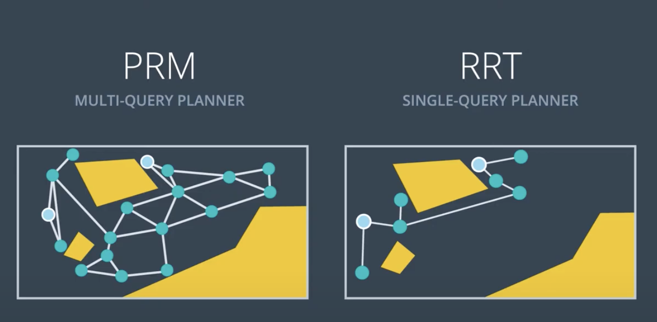
The methods follows start and end. RRT will be explicitly considered from the start.

Then, build up a representation of the workspace. While the PRM build up a graph, RRT will build a tree. That is a type of graph where each node only has one parent. In a single query planner, only concered about getting from start to goal.

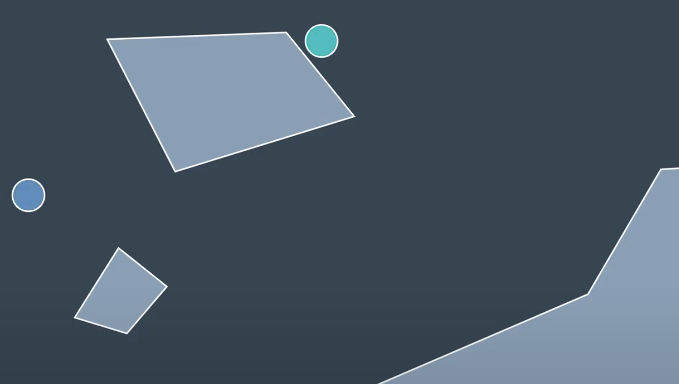
The lack of lateral connections between seemingly neighboring nodes is less of a concern as see below.

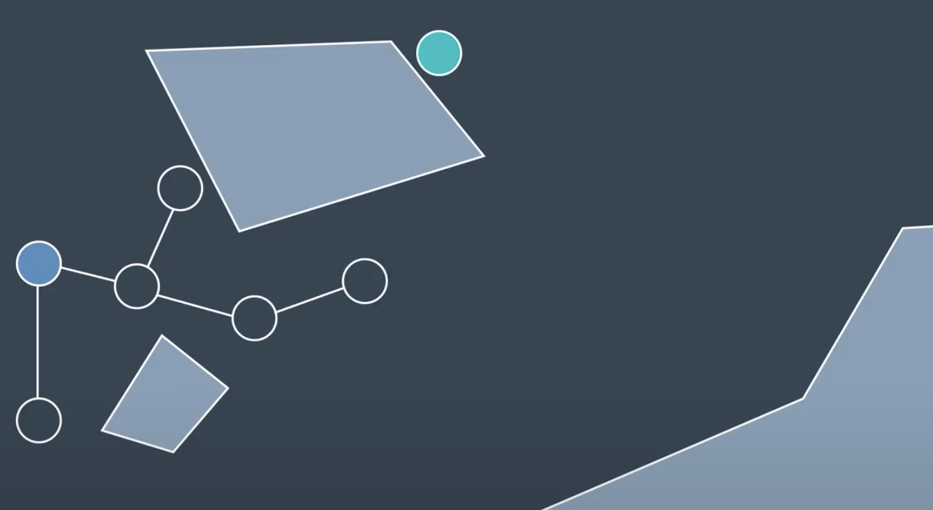
RRT will randomly generate a node, then find its closest neighbor.

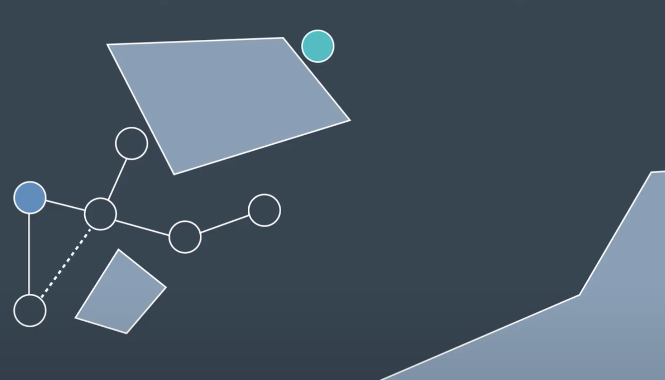
If the nodes whithin a certain distance, delta of the neighbor, then it can be connected directly if the local planner determine the edge to be collision-free.

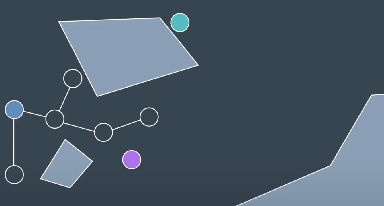
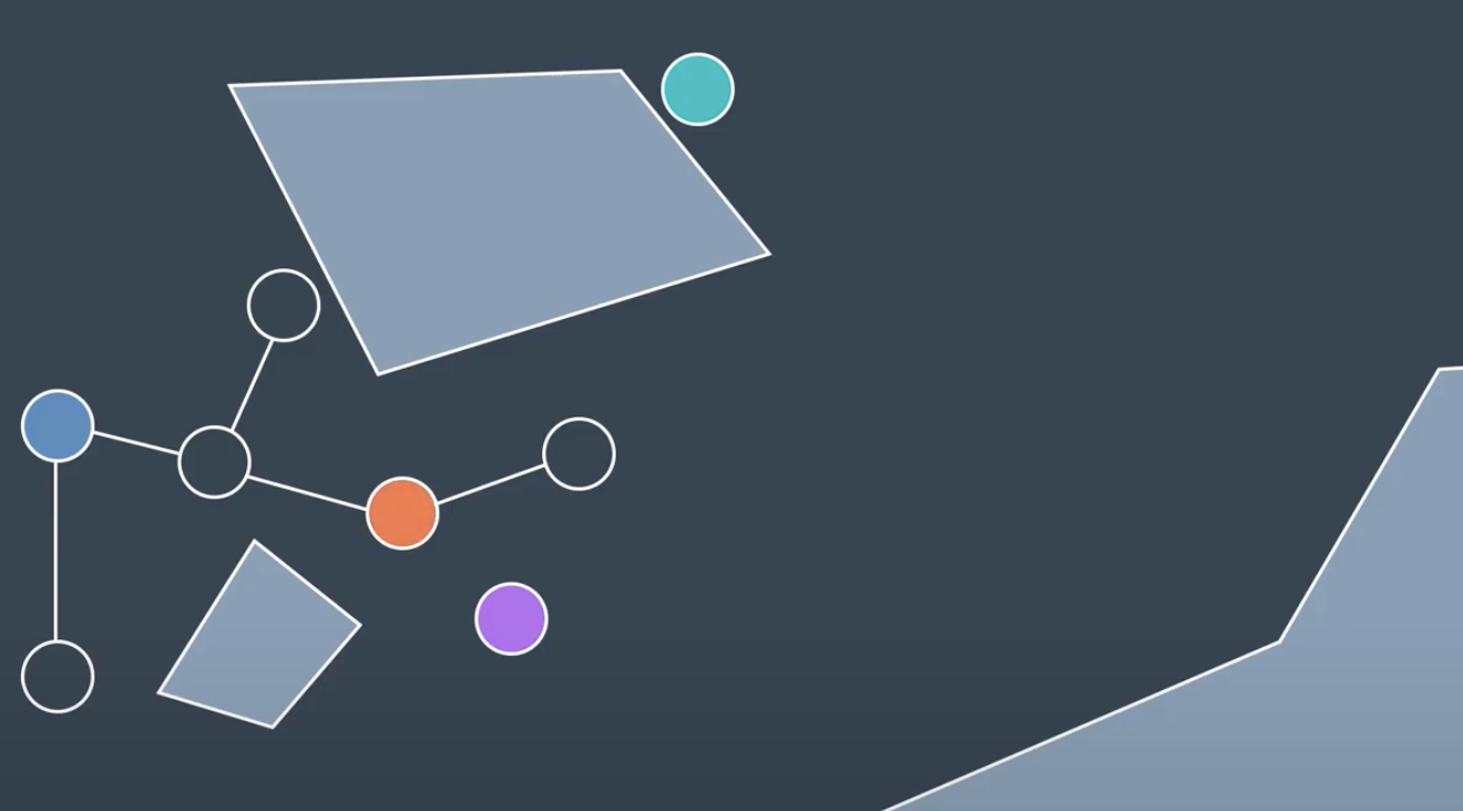
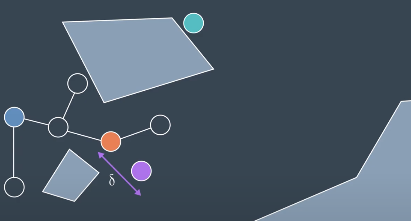
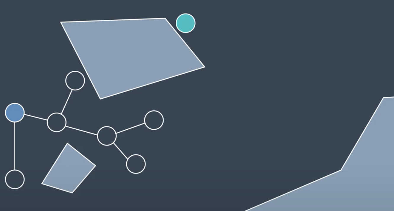
If a newly generated node is a far distance away from all other nodes, then the chance of the edge between the node and its nearest neighbor being collision-free is unlikely. In such a case, instead of connecting to the node, RRT will create a new node in the same direction but a distance delta away. Then it will check for collision and if it's in the clear, the node is added to the tree.

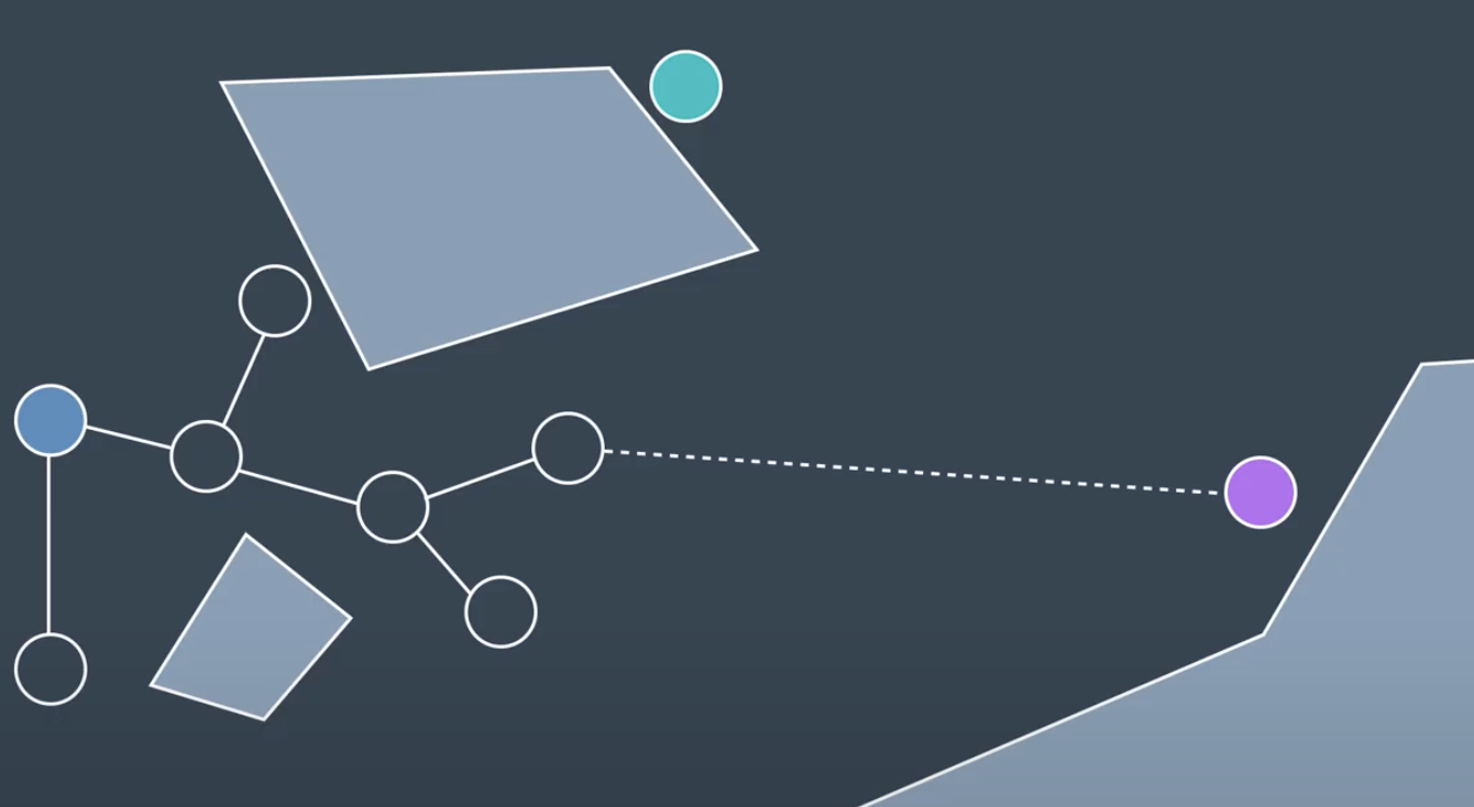
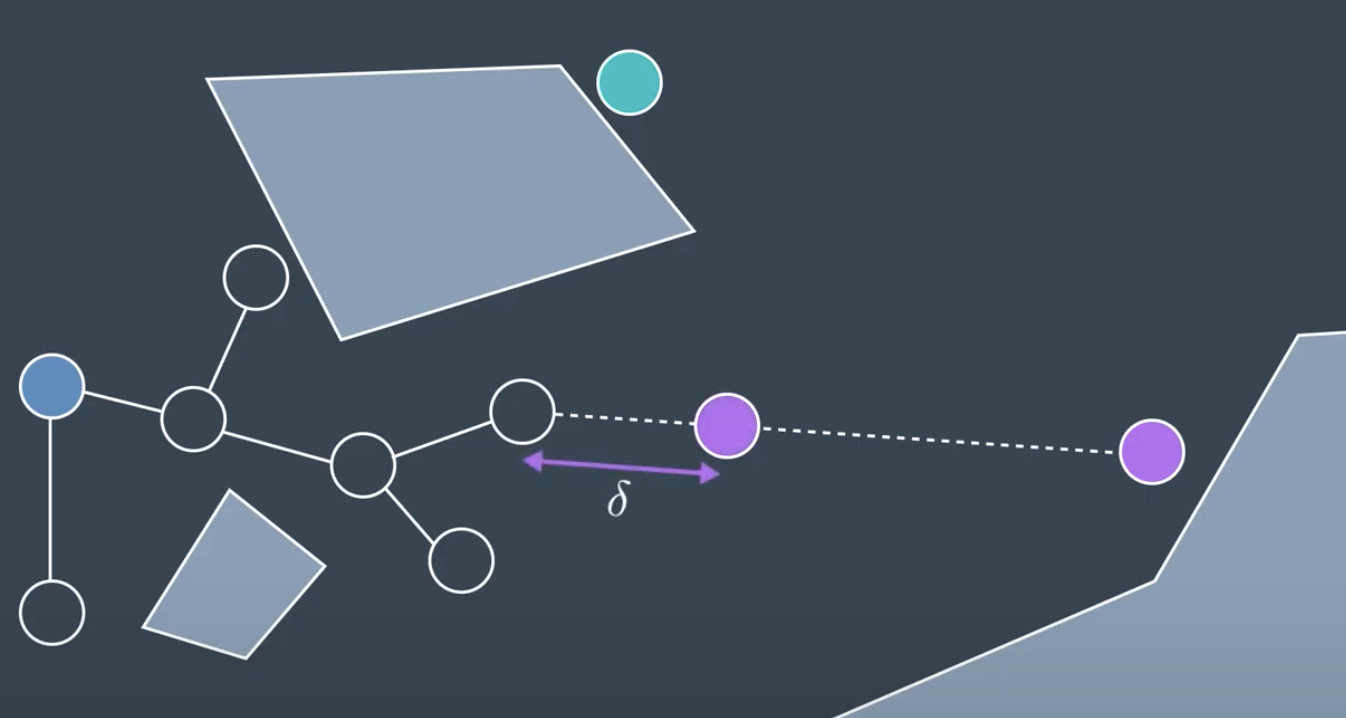
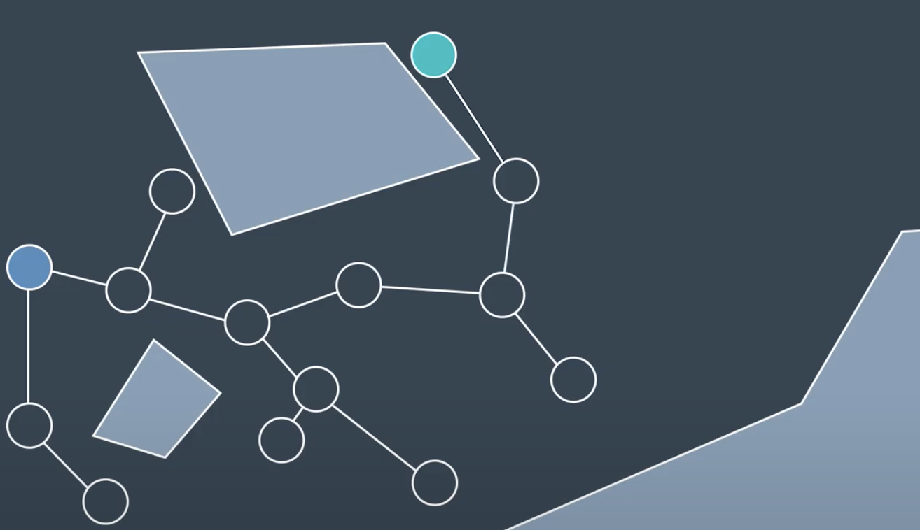
This method is slightly biasing. Therefore, one variation of the RRT method is onee that grows two trees. Onee from thee start and one from the goal. It tries to build an edge between the most recently added node and other tree.

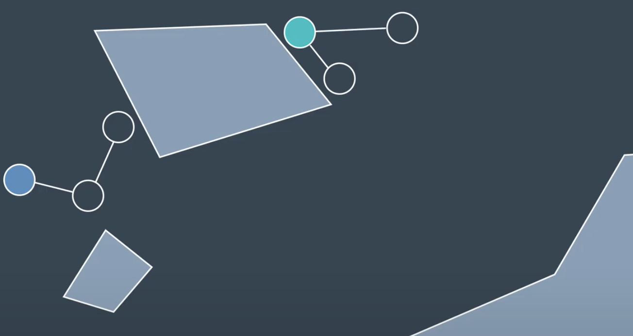
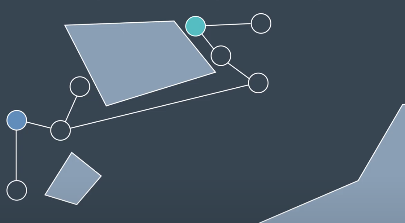
Algorithm pseudocode for the RRT learning phase:

Initialize two empty trees.
Add start node to tree #1.
Add goal node to tree #2.
For n iterations, or until an edge connects trees #1 & #2:

    Generate a random configuration (alternating trees).
    If the configuration is collision free: 
        Find the closest neighbour on the tree to the configuration 
        If the configuration is less than a distance $$\delta$$ away from the neighbour:
            Try to connect the two with a local planner.
    Else:
        Replace the randomly generated configuration 
            with a new configuration that falls along the same path, 
            but a distance $$\delta$$ from the neighbour.
        Try to connect the two with a local planner. 

    If node is added successfully: 
        Try to connect the new node to the closest neighbour.

Setting Parameters

• Sampling method (ie. how a random configuration is generated). As discussed in the video, you can sample uniformly - which would favour wide unexplored spaces, or you can sample with a bias - which would cause the search to advance greedily in the direction of the goal. Greediness can be beneficial in simple planning problems, however in some environments it can cause the robot to get stuck in a local minima. It is common to utilize a uniform sampling method with a small hint of bias.

• Tuned $\delta$. As RRT starts to generate random configurations, a large proportion of these configurations will lie further than a distance $\delta$ from the closest configuration in the graph. In such a situation, a randomly generated node will dictate the direction of growth, while $\delta$ is the growth rate.

• Choosing a small $\delta$ will result in a large density of nodes and small growth rate. On the other hand, choosing a large $\delta$ may result in lost detail, as well as an increasing number of nodes being unable to connect to the graph due to the greater chance of collisions with obstacles. $\delta$ must be chosen carefully, with knowledge of the environment and requirements of the solution.

Single-Query Planner

Since the RRT method explores the graph starting with the start and goal nodes, the resultant graph cannot be applied to solve additional queries. RRT is a single-query planner.

RRT is, however, much quicker than PRM at solving a path planning problem. This is so because it takes into account the start and end nodes, and limits growth to the area surrounding the existing graph instead of reaching out into all distant corners, the way PRM does. RRT is more efficient than PRM at solving large path planning problems in dynamic environments.

RRT is able to solve problems with 7 dimensions in a matter of milliseconds, and may take several minutes to solve problems with over 20 dimensions. In comparison, such problems would be impossible to solve with the combinatorial path planning method.

RRT & Non-holonomic Systems

RRT method supports planning for non-holonomic systems, while the PRM method does not. This is so because the RRT method can take into consideration the additional constraints (such as a car’s turning radius at a particular speed) when adding nodes to a graph, the same way it already takes into consideration how far away a new node is from an existing tree.

Path Smoothing

Instead of using path directly, some post-processing can be applied to smooth out the paths and improve the result. Connecting two non-neighboring nodes together. If it is able to find pair of nodes whose edges is collision free, then the original path between the two nodes is replaced with the shortcut eedge

Algorithm: Method for smoothing the path by shortcutting

For n iterations:
    Select two nodes from the graph
    If the edge between the two nodes is shorter than the existing path between the nodes:
        Use local planner to see if edge is collision-free. 
            If collision-free:
                Replace existing path with edge between the two nodes.

Keep in mind that the path’s distance is not the only thing that can be optimized by the Path Shortcutter algorithm - it could optimize for path smoothness, expected energy use by the robot, safety, or any other measurable factor.

After the Path Shortcutting algorithm is applied, the result is a more optimized path. It may still not be the optimal path, but it should have at the very least moved towards a local minimum. There exist more complex, informed algorithms that can improve the performance of the Path Shortcutter. These are able to use information about the workspace to better guide the algorithm to a more optimal solution.

For large multi-dimensional problems, it is not uncommon for the time taken to optimize a path to exceed the time taken to search for a feasible solution in the first place.

Probabilistic Path Planning

While the first two approaches looked at the path planning problem generically - with no understanding of who or what may be executing the actions - probabilistic path planning takes into account the uncertainty of the robot’s motion. It's used in reinforcement learning as well such as reward.

Probabilistic path planning using Markov decision processes.

Markov Decision Process

Recycling Robot Example

Let's say we have a recycling robot, as an example. The robot’s goal is to drive around its environment and pick up as many cans as possible. It has a set of states that it could be in, and a set of actions that it could take. The robot receives a reward for picking up cans; however, it can also receive a negative reward (a penalty) if it runs out of battery and get stranded.

The robot has a non-deterministic transition model (sometimes called the one-step dynamics). This means that an action cannot guarantee to lead a robot from one state to another state. Instead, there is a probability associated with resulting in each state.

Say at an arbitrary time step t, the state of the robot's battery is high ($S_{t} = high$). In response, the agent decides to search for cans ($A_{t} = search$). in such a case, there is a 70% chance of the robot’s battery charge remaining high and a 30% chance that it will drop to low.

MDP Definition

A Markov Decision Process is defined by:

• A set of states: $S$
• Initial state: $s_{0}$
• A set of actions: $A$
• The transition model: $T(s,a,s')$
• A set of rewards: $R$

The transition model is the probability of reaching a state s' from a statee s by executing action a. It is often written as T(s,a,s')

The Markov assumption states that the probability of transitioning from s to s' is only dependent on the present state, s, and not on the path taken to get to s.

One notable difference between MDPs in probabilistic path planning and MDPs in reinforcement learning (RL), is that in path planning the robot is fully aware of all of the items listed above (state, actions, transition model, rewards). Whereas in RL, the robot was aware of its state and what actions it had available, but it was not aware of the rewards or the transition model.

Mobile Robot Example

In movement actions are non-deterministic, every action will have a probability less than 1 of being successfully executed. This can be due to a number of reasons such as wheel slip, internal errors, difficult terrain, etc. The image below showcases a possible transition model for our exploratory rover, for a scenario where it is trying to move forward one cell. 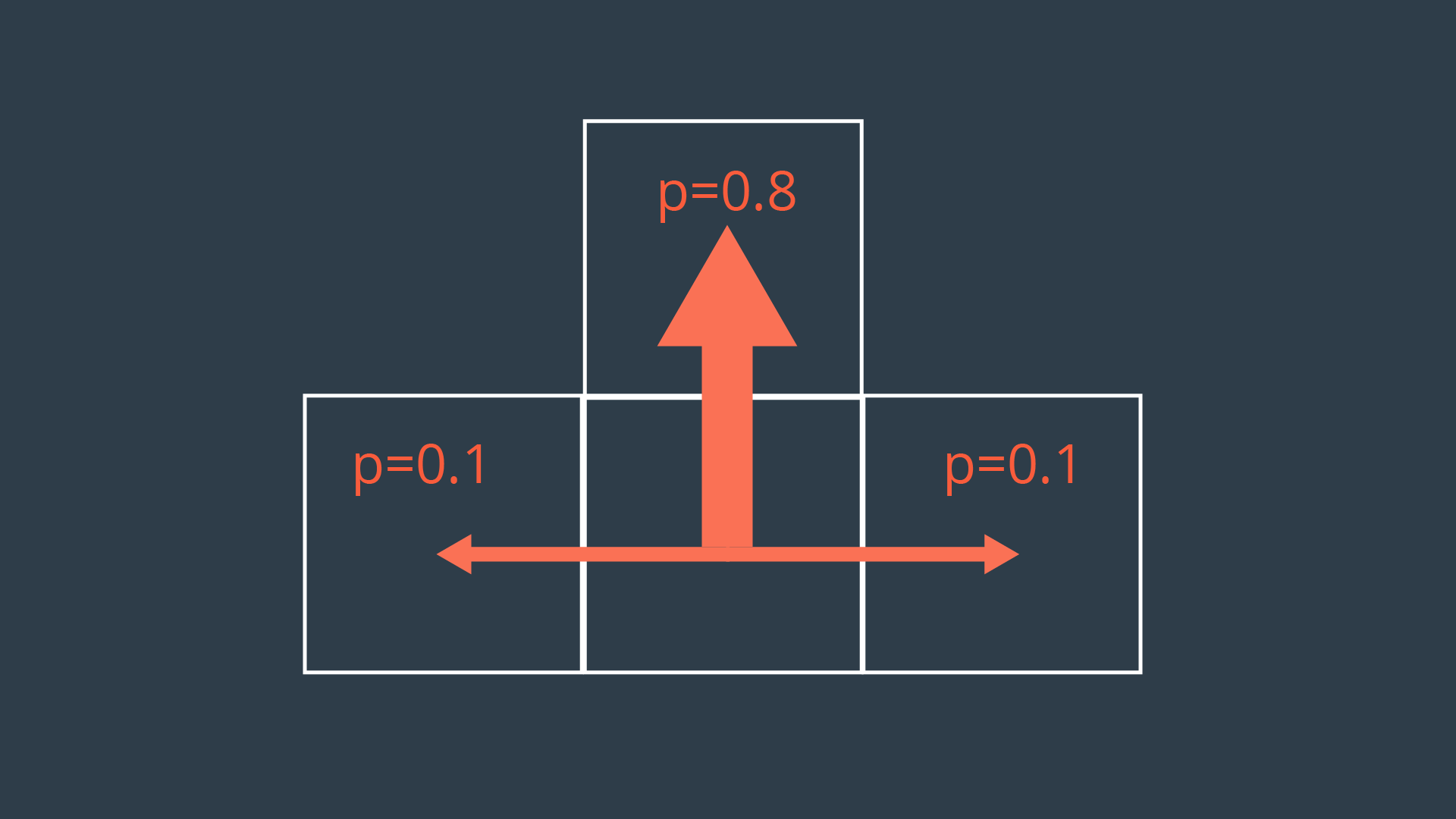As you can see, the intended action of moving forward one cell is only executed with a probability of 0.8 (80%). With a probability of 0.1 (10%), the rover will move left, or right. Let’s also say that bumping into a wall will cause the robot to remain in its present cell.

Let’s provide the rover with a simple example of an environment for it to plan a path in. The environment shown below has the robot starting in the top left cell, and the robot’s goal is in the bottom right cell. The mountains represent terrain that is more difficult to pass, while the pond is a hazard to the robot. Moving across the mountains will take the rover longer than moving on flat land, and moving into the pond may drown and short circuit the robot.

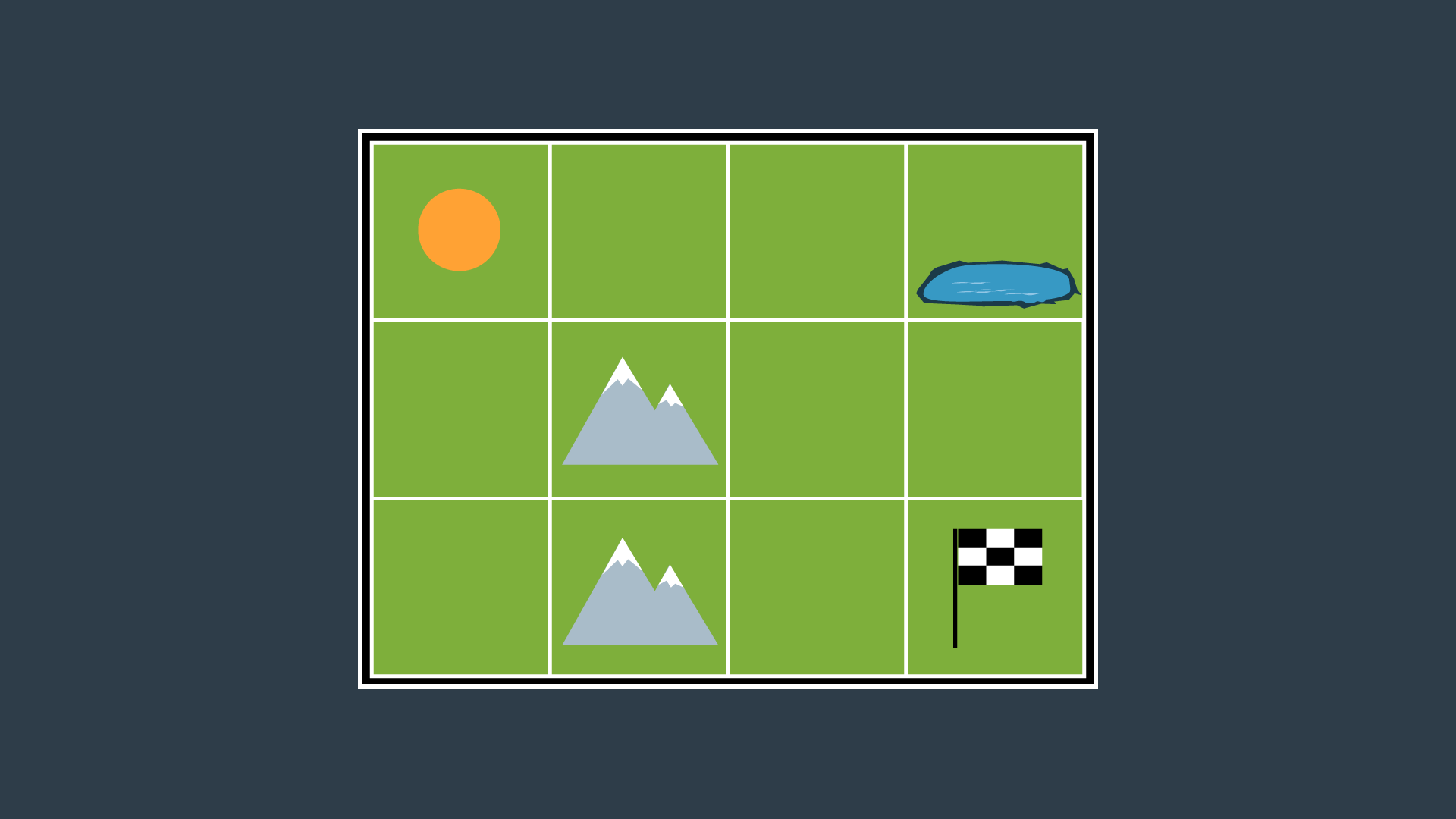
Combinatorial Path Planning Solution

If we were to apply A* search to this discretized 4-connected environment, the resultant path would have the robot move right 2 cells, then down 2 cells, and right once more to reach the goal (or R-R-D-R-D, which is an equally optimal path). This truly is the shortest path, however, it takes the robot right by a very dangerous area (the pond). There is a significant chance that the robot will end up in the pond, failing its mission. If we are to path plan using MDPs, we might be able to get a better result!

Probabilistic Path Planning Solution

In each state (cell), the robot will receive a certain reward, $R$(s). This reward could be positive or negative, but it cannot be infinite. It is common to provide the following rewards,

• Small negative rewards to states that are not the goal state(s) - to represent the cost of time passing (a slow moving robot would incur a greater penalty than a speedy robot)
• Large positive rewards for the goal state(s)
• Large negative rewards for hazardous states - in hopes of convincing the robot to avoid them.

These rewards will help guide the rover to a path that is efficient, but also safe - taking into account the uncertainty of the rover’s motion.

The image below displays the environment with appropriate rewards assigned. 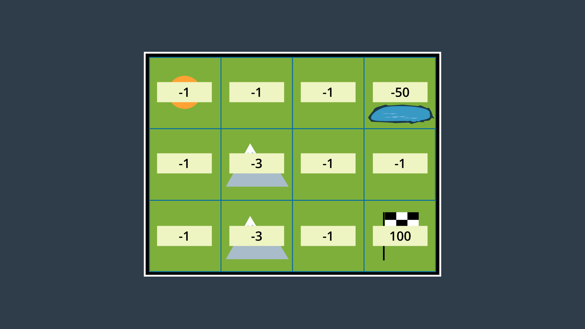As you can see, entering a state that is not the goal state has a reward of -1 if it is a flat-land tile, and -3 if it is a mountainous tile. The hazardous pond has a reward of -50, and the goal has a reward of 100.

With the robot’s transition model identified and appropriate rewards assigned to all areas of the environment, we can now construct a policy. Read on to see how that’s done in probabilistic path planning!

Policies

Solution to a Markov Decision Process is called a policy, and is denoted with the letter π.

Definition

A policy is a mapping from states to actions. For every state, a policy will inform the robot of which action it should take. An optimal policy, denoted π*, informs the robot of the best action to take from any state, to maximize the overall reward. It is highly recommended that you are familiar with the basics of Reinforcement Learning (RL), ie. what a policy is, how state-value is calculated, and how the Bellman equations can be used to compute the optimal policy. Go through these RL concepts to solve gridworld problem.

Developing a Policy

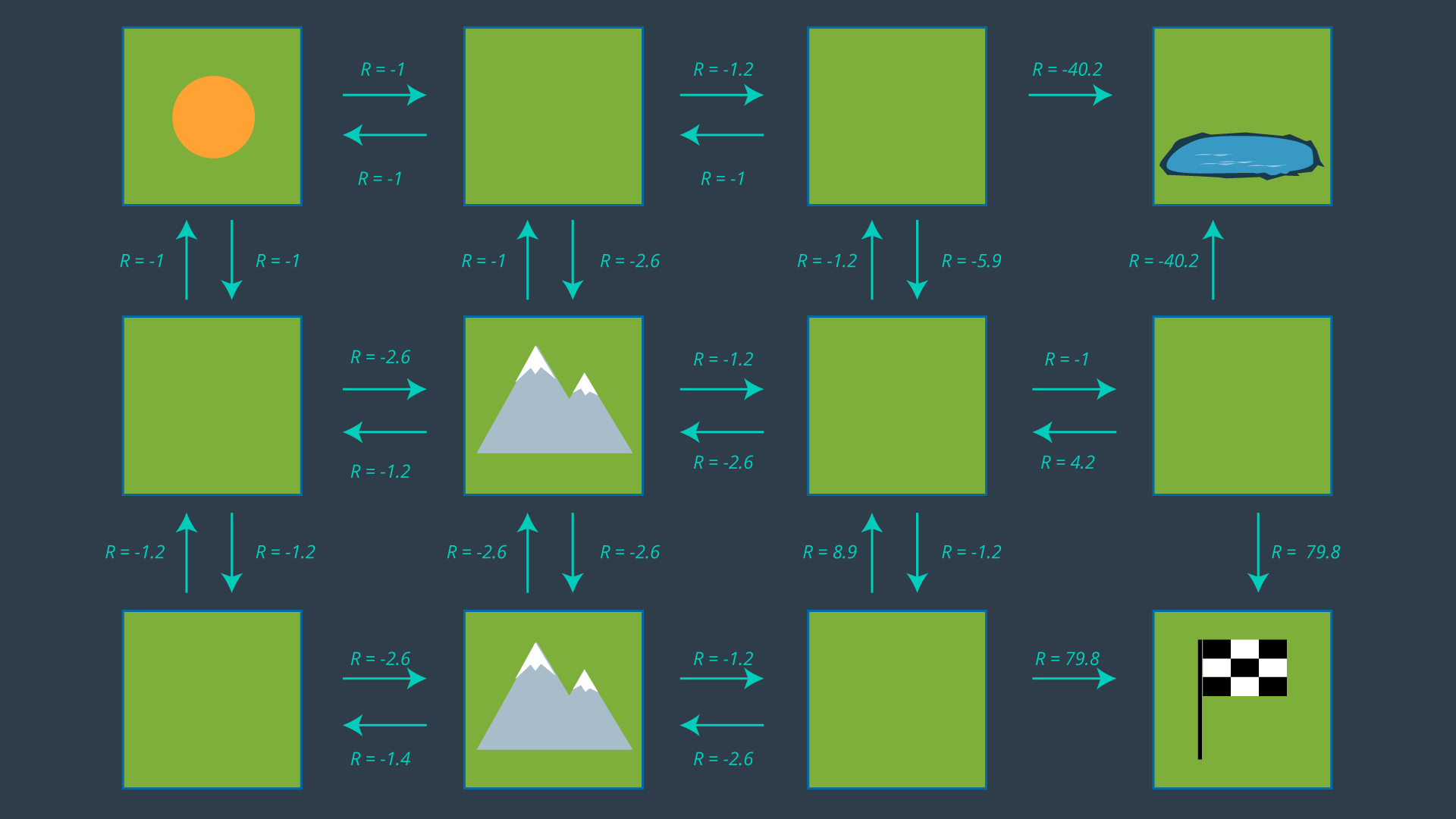
The image below displays the set of actions that the robot can take in its environment. Note that there are no arrows leading away from the pond, as the robot is considered DOA (dead on arrival) after entering the pond. As well, no arrows leave the goal as the path planning problem is complete once the robot reaches the goal - after all, this is an episodic task. 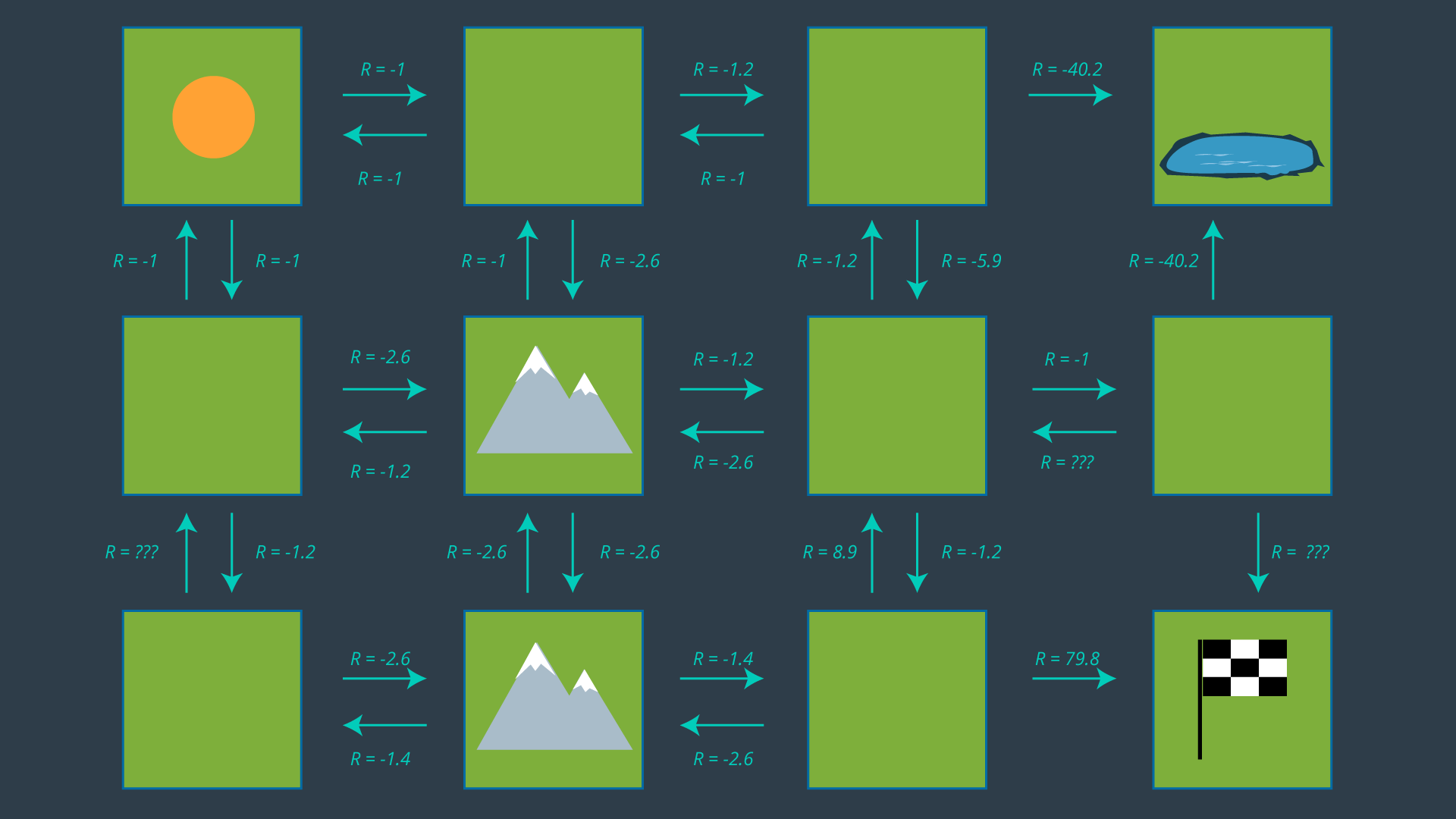From this set of actions, a policy can be generated by selecting one action per state. Before we revisit the process of selecting the appropriate action for each policy, let’s look at how some of the values above were calculated. After all, -5.9 seems like quite an odd number!

Calculating Expected Rewards

Recall that the reward for entering an empty cell is -1, a mountainous cell -3, the pond -50, and the goal +100. These are the rewards defined according to the environment. However, if our robot wanted to move from one cell to another, it it not guaranteed to succeed. Therefore, we must calculate the expected reward, which takes into account not just the rewards set by the environment, but the robot's transition model too.

Let’s look at the bottom mountain cell first. From here, it is intuitively obvious that moving right is the best action to take, so let’s calculate that one. If the robot’s movements were deterministic, the cost of this movement would be trivial (moving to an open cell has a reward of -1). However, since our movements are non-deterministic, we need to evaluate the expected reward of this movement. The robot has a probability of 0.8 of successfully moving to the open cell, a probability of 0.1 of moving to the cell above, and a probability of 0.1 of bumping into the wall and remaining in its present cell.

$expected$ $reward = 0.8*(−1)+0.1*(−3)+0.1*(−3) = -1.4$

All of the expected rewards are calculated in this way, taking into account the transition model for this particular robot.

Selecting a Policy

Now that we have an understanding of our expected rewards, we can select a policy and evaluate how efficient it is. Once again, a policy is just a mapping from states to actions. If we review the set of actions depicted in the image above, and select just one action for each state - i.e. exactly one arrow leaving each cell (with the exception of the hazard and goal states) - then we have ourselves a policy.

However, we’re not looking for any policy, we’d like to find the optimal policy. For this reason, we’ll need to study the utility of each state to then determine the best action to take from each state.

State Utility

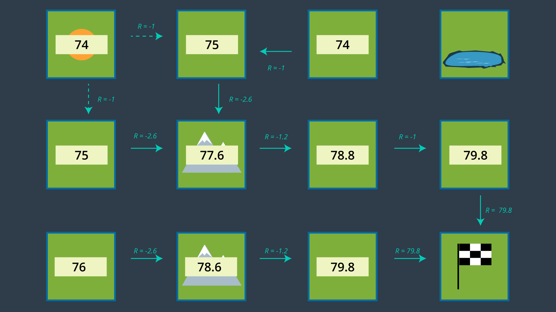
The utility of a state (otherwise known as the state-value) represents how attractive the state is with respect to the goal. Recall that for each state, the state-value function yields the expected return, if the agent (robot) starts in that state and then follows the policy for all time steps. In mathematical notation, this can be represented as so:

$U^{\pi}(s)$ = $E$[ $∑_{t=0}^{∞}$ $R(s_{t})|\pi, s_{0}=s$]

• $U^{\pi}(s)$ : Utility of a state s
• $E$ : expected value
• $R(s)$ : reward for state s

The utility of a state is the sum of the rewards that an agent would encounter if it started at that state and followed the policy to the goal.

$U^{\pi}(s)$ = $E$[ $∑_{t=0}^{∞}$ $R(s_{t})|\pi, s_{0}=s$]

$U^{\pi}(s)$ = R(s) + $E$[ $∑_{t=0}^{∞}$ $R(s_{t})|\pi, s_{0}=s$']

$U^{\pi}(s)$ = R(s) + $U^{\pi}(s')$

Determining the Optimal Policy

Recall that the optimal policy, denoted, $\pi^{*}$, informs the robot of the best action to take from any state, to maximize the overall reward

$\pi^{*}(s) = argmax E$ [ $U^{\pi}(s)$ ]

In a state s, the optimal policy $\pi^{*}$ will choose the action a that maximizes the utility of s (which, due to its iterative nature, maximizes the utilities of all future states too). While the math may make it seem intimidating, it’s as easy as looking at the set of actions and choosing the best action for every state.

The process of selecting each state’s most rewarding action continues, until every state is mapped to an action. These mappings are precisely what make up the policy.

Applying the Policy

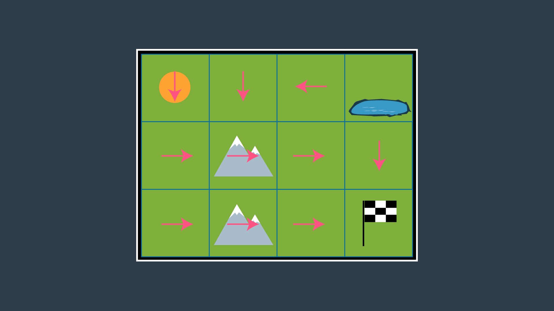
Once this process is complete, the agent (our robot) will be able to make the best path planning decision from every state, and successfully navigate the environment from any start position to the goal. The optimal policy for this environment and this robot is provided below.

The image below that shows the set of actions with just the optimal actions remaining. Note that from the top left cell, the agent could either go down or right, as both options have equal rewards.

Discounting

One simplification that you may have noticed us make, is omit the discounting rate $\gamma$. In the above example, $\gamma = 1$s and all future actions were considered to be just as significant as the present action. This was done solely to simplify the example.

In reality, discounting is often applied in robotic path planning, since the future can be quite uncertain. The complete equation for the utility of a state is provided below: $U^{\pi}(s)$ = $E$[ $∑_{t=0}^{∞}$ $\gamma$ $R(s_{t})|\pi, s_{0}=s$]

Value Iteration Algorithm

The process that we went through to determine the optimal policy for the mountainous environment was fairly straightforward, but it did take some intuition to identify which action was optimal for every state. In larger more complex environments, intuition may not be sufficient. In such environments, an algorithm should be applied to handle all computations and find the optimal solution to an MDP. One such algorithm is called the Value Iteration algorithm.

The Value Iteration algorithm will initialize all state utilities to some arbitrary value - say, zero. Then, it will iteratively calculate a more accurate state utility for each state, using

$U(s) = R(s)+$ $\gamma$ $max_{a}$ $Σ_{s'}$ $T(s,a,s')U(s')$

Algorithm

U' = 0
loop until close-enough(U, U')
    U = U'
    for s in S, do:
        U(s) = R(s) + \gamma max_{a} Σ_{s'} T(s,a,s')U(s')
return U

With every iteration, the algorithm will have a more and more accurate estimate of each state’s utility. The number of iterations of the algorithm is dictated by a function close-enough which detects convergence. One way to accomplish this is to evaluate the root mean square error,

$RMS = 1/|s| * \sqrt(Σ_{s} (U(s)-U'(s))^2)$

Once this error is below a predetermined threshold, the result has converged sufficiently.

RMA(U, U') < ϵ

This algorithm finds the optimal policy to the MDP, regardless of what U' is is initialized to (although the efficiency of the algorithm will be affected by a poor U')

Review

Discrete Path Planning

• Continuous Representation

  • Create a configuration space.

• Discretization

  • Three different types of methods used to represent a configuration space with discrete segments.
    • Roadmap group of methods: Modeled the configuration space as a simple graph by either connecting the vertices of the obstacles or building a Voronoi diagram.
    • Cell Decomposition: Broke the space into a finite number of cells, each of which was assessed to be empty, full, or mixed. The empty cells will linked together to create a graph.
    • Gradient field: Method that models the configuration space using a 3D function that has the goal as global minimum and obstacles as tall structures.

• Graph Search

  • A* Searchadmissibility is a requirement for A* to be optimal. For this reason, common heuristics include the Euclidean distance from a node to the goal, or in some applications the Manhattan distance. When comparing two different types of values - for instance, if the path cost is measured in hours, but the heuristic function is estimating distance - then you would need to determine a scaling parameter to be able to sum the two in a useful manner.
  • A* search hueristic guide
  • Path Finding Visualization
  • MovingAI A* Variance
  • Variants of A* - Stanford

• Anytime algorithm: an anytime algorithm is an algorithm that will return a solution even if it's computation is halted before it finishes searching the entire space. The longer the algorithm plans, the more optimal the solution will be.

• RRT*: RRT* is a variant of RRT that tries to smooth the tree branches at every step. It does so by looking to see whether a child node can be swapped with it's parent (or it's parent's parent, etc) to produce a more direct path. The result is a less zig-zaggy and more optimal path.

Path Planning for Non-Circular Micro Aerial Vehicles in Constrained Environmentss

Reinforcement Learning

• Wikipedia - Reinforcement Learning
• Reinforcement Learning 101 - solve the gridworld state-value function