ml-plot-utils

MATLAB scripts to facilitate common plotting tasks for dynamical systems simulations. All the plots use Latex fonts.

Examples

1. Input-output plots for a dynamic system

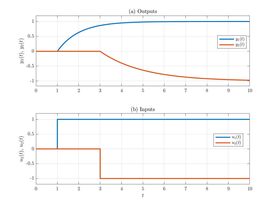
% Simulate continuous-time 2x2 system
t = linspace(0, 10, 101)';
nT = size(t, 1) - 1;
U = zeros(nT+1,2);
U(t >= 1, 1) = 1;
U(t >= 3, 2) = -1;
G = [tf(1, [1 1]) 0;
     0            tf(1, [2 1])];
[Y, t] = lsim(G,U,t);
u_labels = {'$u_1(t)$', '$u_2(t)$'};  % or ["$u_1(t)$" "$u_2(t)$"]
y_labels = {'$y_1(t)$', '$y_2(t)$'};

% Make input-output plot
figure
make_ioplot(Y, t, U, u_labels, y_labels)

% Save plot as pdf file
save_fig_to_pdf('plots/ioplot3.pdf')

2. Step response plots

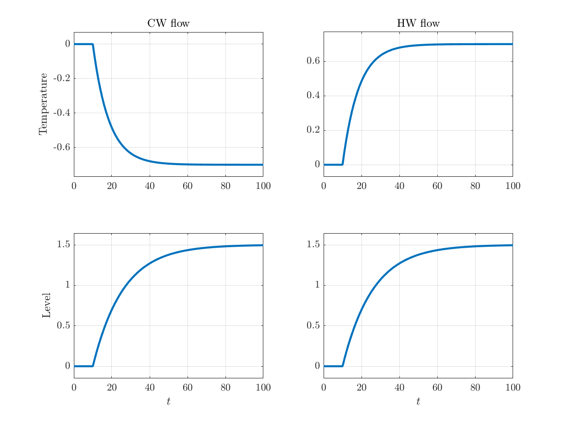
Make a matrix of the step responses of SISO or MIMO linear systems. Similar to MATLAB's built-in step plot function but with more control over formatting and labelling.

% Define 2x2 system
s = tf('s');
G11 = -0.7 / (1 + 8.5*s);
G12 = -G11;
G21 = 1.5 / (1 + 16*s);
G22 = G21;
Gc = [G11 G12; G21 G22];
Gc.InputName = ["CW flow", "HW flow"];
Gc.OutputName = ["Temperature", "Level"];

% Make into discrete system
Ts = 1;
Gd = c2d(Gc,Ts,'zoh');

% Plot step responses
figure(8)
nT = 100;
t = Ts*(0:nT)';
make_stepresp_plots(Gd, t)
save_fig_to_pdf('plots/stepresp_plots.pdf')

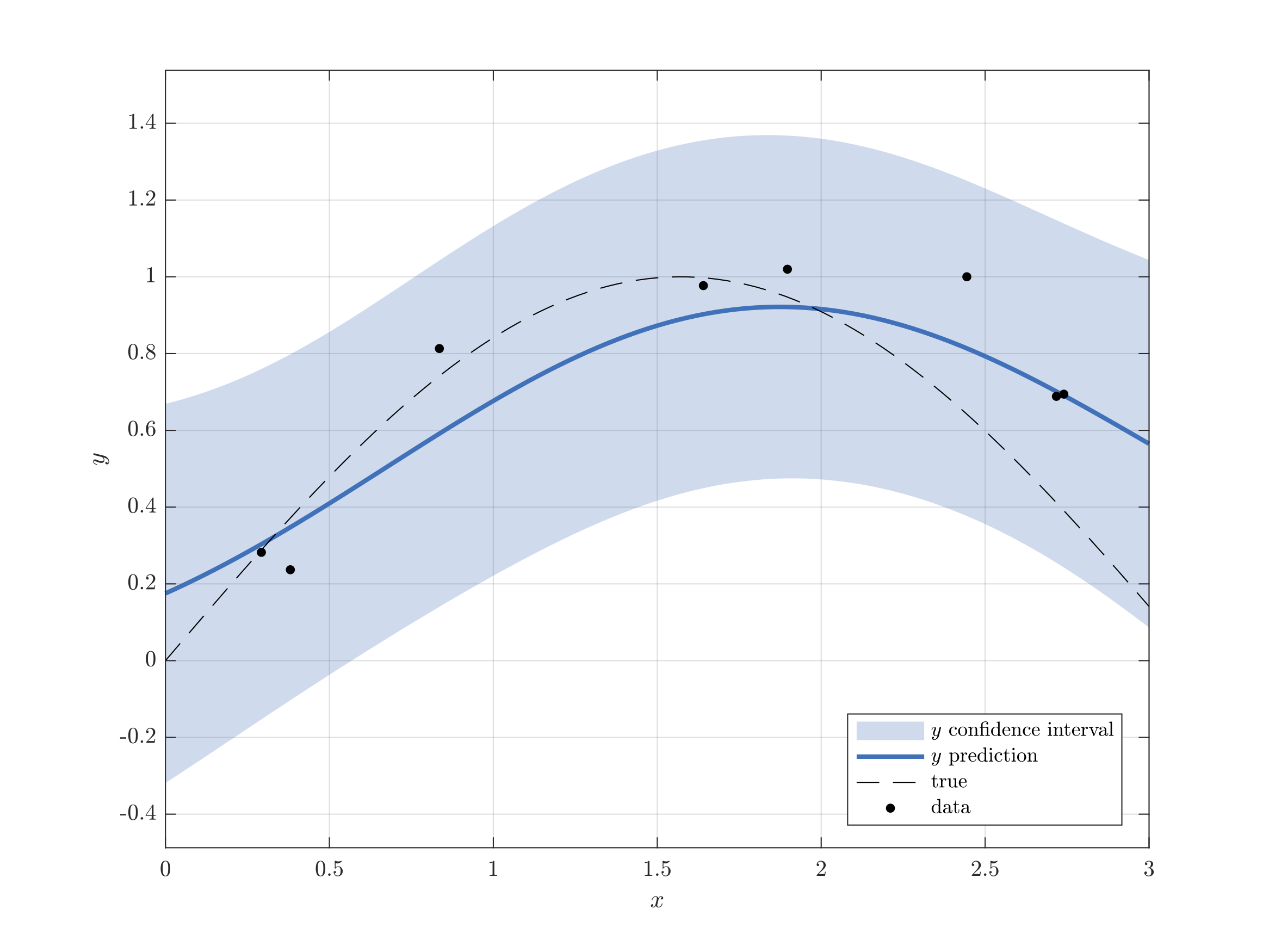
3. Statistical plot of probabilistic model predictions

These are useful for comparing the predictions of probabilistic models, such as a Gaussian process model, with the data and/or with the true values if known.

rng(0);

% Function to model
f = @sin;

% Generate data sample
n = 8;
sigma_M = 0.1;  % measurement noise
x_d = rand(n, 1)*3;
y_d = sin(x_d) + sigma_M*randn(n, 1);

% Fit Gaussian process model
sigmaL0 = 1;  % Length scale for predictors
sigmaF0 = 0.3;  % Signal standard deviation
sigmaN0 = 0.2;  % Initial noise standard deviation
gpr_model = fitrgp(x_d, y_d, 'FitMethod', 'none', ...
    'KernelParameters', [sigmaL0; sigmaF0], 'Sigma', sigmaN0);

% Make new predictions with model
x = linspace(0, 3, 101)';
[Y_pred, ~, Y_pred_int] = predict(gpr_model, x);

% True values
y_true = f(x);

% Plot predictions compared to true values and data
figure
make_stattdplot(Y_pred, Y_pred_int(:, 1), Y_pred_int(:, 2), y_true, x, ...
   y_d, x_d, "$x$", "$y$", "prediction", "confidence interval")
save_fig_to_pdf('plots/stattdplot1.pdf')

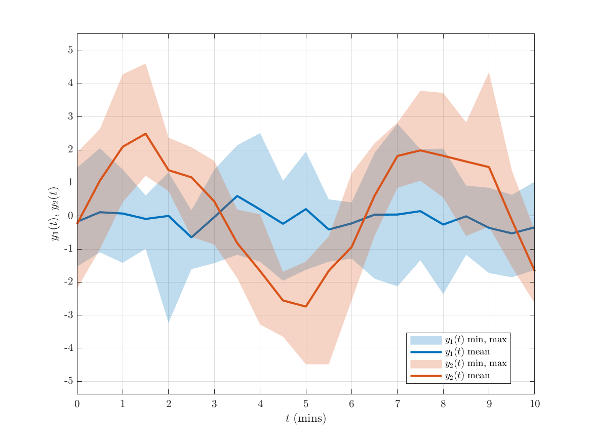
4. Time-series plot of the statistics of a group of signals.

% Generate two groups of 10 random signals
t = 0.5*(0:20)';
Y = {randn(21, 10), randn(21, 10)+2*sin(t)};

% Make statistics plot
figure
y_labels = {'$y_1(t)$', '$y_2(t)$'};
make_tsstatplot(Y, t, y_labels, '$t$ (mins)', nan(2), 'minmax', 'mean')

% Save plot as pdf file
save_fig_to_pdf('plots/tsstatplot4.pdf')

3. Correlograms

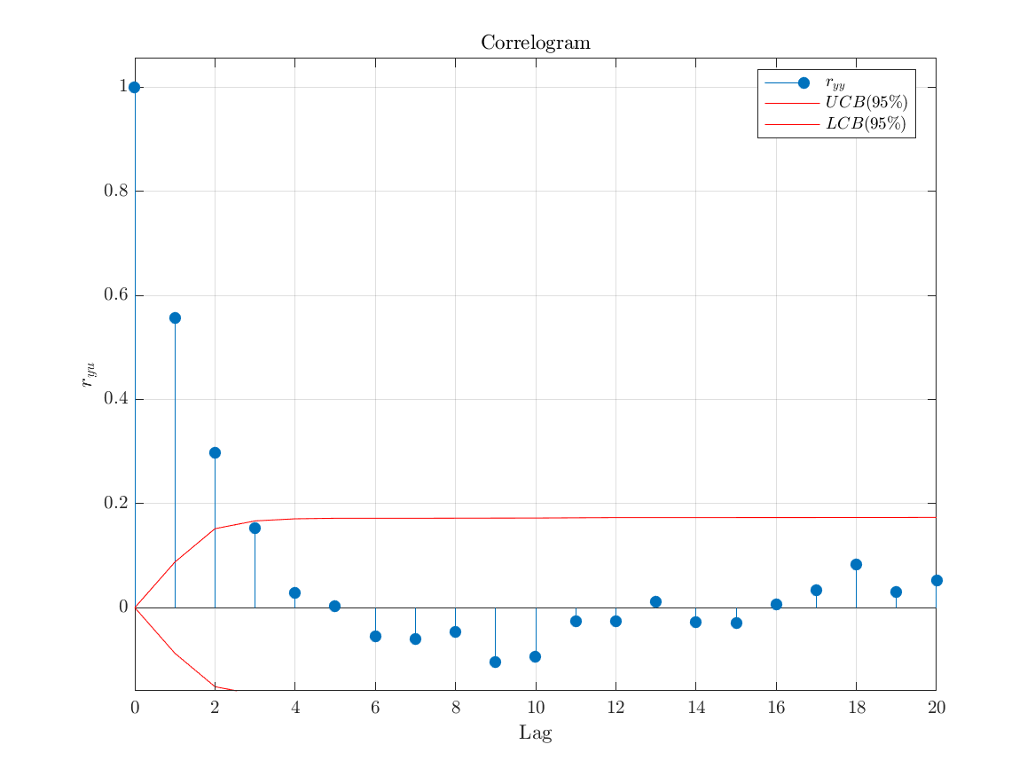
Auto-correlogram plot with confidence bounds:

data = readtable('test_data/tsdata1.csv');

figure
plot_correlogram_auto_conf(data.y4)
save_fig_to_pdf('plots/corrplot1.pdf')

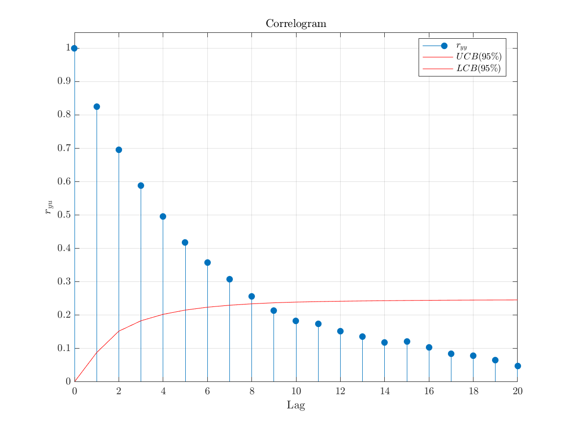
Cross-correlogram plot with confidence bounds:

data = readtable('test_data/tsdata2.csv');

figure
plot_correlogram_auto_conf(data.y2)
save_fig_to_pdf('plots/corrplot2.pdf')

Full list of functions

Main plot functions

make_tsplot.m - Single time series plot of one or more signals
make_ioplot.m - Two time series plots of input and output signals
make_iorplot.m - Two time series plots of input, output and reference signals
make_iodplot.m - Two time series plots of input signal, true output signal, and measured output data
make_iodmplot.m - Two time series plots of input signal, true output signal, measured output data, and model output
make_statplot.m - x-y plot of a probabilistic model(s) (incl. the mean or median value, and a lower and upper bound)
make_stattplot.m - x-y plot of a probabilistic model(s) compared to the true values
make_statdplot.m - x-y plot of a probabilistic model(s) compared to a set of data points
make_stattdplot.m - x-y plot of a probabilistic model compared to true value and the data points
make_tsstatplot.m - Time-series plot of mean (or median), lower, and upper bounds of one or more groups of signals
plot_correlogram_auto_conf.m - Correlogram of auto-correlation coefficients incl. confidence limits
plot_correlogram_x_with_conf.m - Correlogram of cross-correlation coefficients incl. confidence limits
plot_ratios_of_corr_coefficients.m - Bar plot of ratios of consecutive correlation coefficients
show_waterfall_plot.m - Waterfall plot of multiple time series
make_stepresp_plot.m - Step response plot of a SISO dynamical system
make_stepresp_plots.m - Matrix of response plots of a MIMO dynamical system.
make_area_step_plot.m - Stacked area plot with discrete step changes similar to a stairs plot.

Utility functions

axes_limits_with_margin.m - Calculates new axes limits based on the extreme values in the data with the option to add margins and a minimum range
confidence_intervals_auto.m - Calculate lower and upper confidence limits for auto-correlation coefficients
confidence_intervals_x.m - Calculate lower and upper confidence limits for cross-correlation coefficients
ratios_of_corr_coefficients.m - Calculates the ratios of correlation coefficients
escape_latex_chars.m - Prevents text symbols such as '_' being interpreted as Latex
save_fig_to_pdf.m - Saves a pdf document of the current figure with the paper size adjusted to correct size
string2latex.m - Converts a string or a cell array of strings to latex input format

Test scripts

billtubbs / ml-plot-utils