A python library for performing unsupervised machine learning on datasets with learning (e.g. PCA) in contrastive settings, where one is interested in patterns (e.g. clusters or clines) that exist one dataset, but not the other.
Applications include dicovering subgroups in biological and medical data. Here are basic installation and usage instructions, written for Python 3 (in which the library has been developed and tested, although it should work in Python 2 as well).
For more details, see the accompanying paper: "Exploring Patterns Enriched in a Dataset with Contrastive Principal Component Analysis", Nature Communications (2018), and please use the citation below.
@article{abid2018exploring,
  title={Exploring patterns enriched in a dataset with contrastive principal component analysis},
  author={Abid, Abubakar and Zhang, Martin J and Bagaria, Vivek K and Zou, James},
  journal={Nature communications},
  volume={9},
  number={1},
  pages={2134},
  year={2018},
}
This repository also includes experiments to reproduce most of the figures in the paper. Please see the python notebooks in the experiments folder.
$ pip3 install contrastive
The basic functions enabled by this library are shown below. Generally speaking, we have two datasets, one is a dataset that we can label as foreground_data, which is the dataset in which we are discovering patterns and directions, and another dataset called background_data, which is the dataset that does not have the patterns or directions we are interested in discovering. In some cases, both datasets may contain the signal of interest, but the foreground dataset may have the pattern enriched relative to the background. In these analyses, there is a contrast parameter, known as alpha, which can be thought of as a hyperparameter.
from contrastive import CPCA

mdl = CPCA()
projected_data = mdl.fit_transform(foreground_data, background_data)

#returns a set of 2-dimensional projections of the foreground data stored in the list 'projected_data', for several different values of 'alpha' that are automatically chosen (by default, 4 values of alpha are chosen)
Note that foreground_data and background_data should be 2D numpy arrays that have the second dimension (which represents the number of features). In other words, foreground_data.shape[1]==background_data.shape[1] should return True.
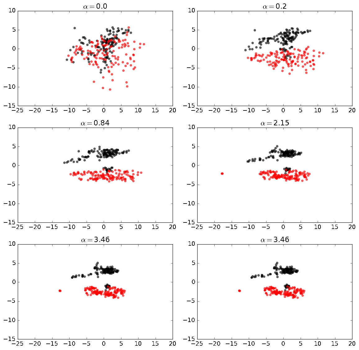
Built-in plotting: to quickly see the results of contrastive PCA, simply enable the plot parameter to true:
from contrastive import CPCA

mdl = CPCA()
projected_data = mdl.fit_transform(foreground_data, background_data, plot=True)
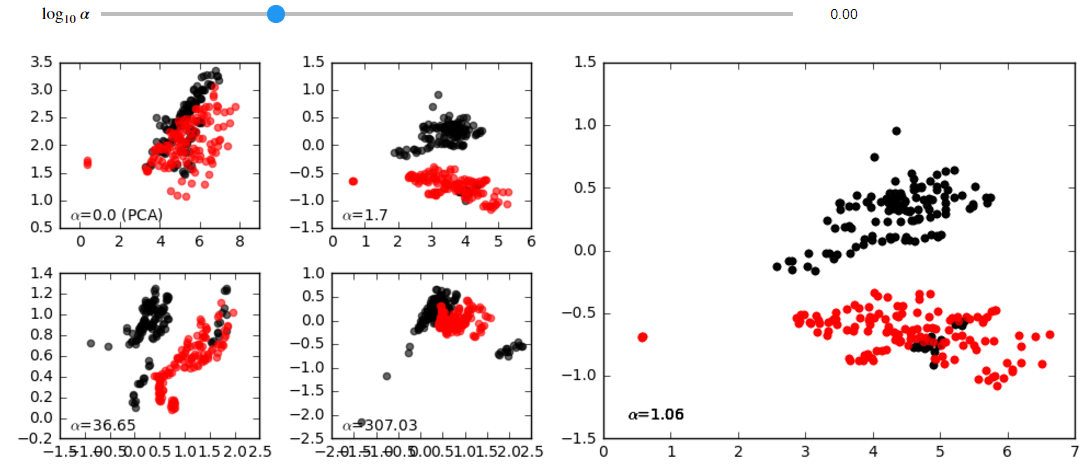
Interactive GUI: if you are running these analyses inside a jupyter notebook, you can easily launch an interactive GUI as shown here:
from contrastive import CPCA

mdl = CPCA()
projected_data = mdl.fit_transform(foreground_data, background_data, gui=True)
Using the slider, you can see how the your data points move as you change the value of the contrast parameter. These animations can reveal groups in the data and other insights:
To ensure that the library is working, here is a quick script that will allow you to test the code on synthetic data. Simply run the following commands:
import numpy as np
from contrastive import CPCA

N = 400; D = 30; gap=3
# In B, all the data pts are from the same distribution, which has different variances in three subspaces.
B = np.zeros((N, D))
B[:,0:10] = np.random.normal(0,10,(N,10))
B[:,10:20] = np.random.normal(0,3,(N,10))
B[:,20:30] = np.random.normal(0,1,(N,10))


# In A there are four clusters.
A = np.zeros((N, D))
A[:,0:10] = np.random.normal(0,10,(N,10))
# group 1
A[0:100, 10:20] = np.random.normal(0,1,(100,10))
A[0:100, 20:30] = np.random.normal(0,1,(100,10))
# group 2
A[100:200, 10:20] = np.random.normal(0,1,(100,10))
A[100:200, 20:30] = np.random.normal(gap,1,(100,10))
# group 3
A[200:300, 10:20] = np.random.normal(2*gap,1,(100,10))
A[200:300, 20:30] = np.random.normal(0,1,(100,10))
# group 4
A[300:400, 10:20] = np.random.normal(2*gap,1,(100,10))
A[300:400, 20:30] = np.random.normal(gap,1,(100,10))
A_labels = [0]*100+[1]*100+[2]*100+[3]*100

cpca = CPCA(standardize=False)
cpca.fit_transform(A, B, plot=True, active_labels=A_labels)
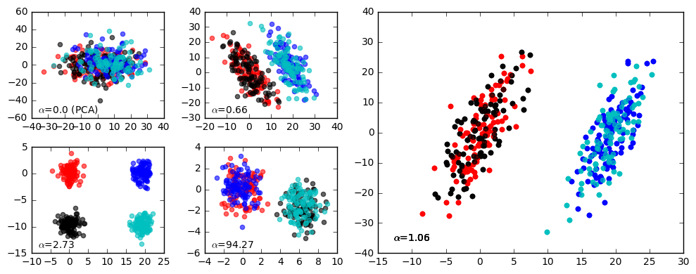
You should see a series of plots that looks something like this:
Labels for foreground data (plot/gui mode): In the examples above, the data points are colored according to labels known ahead of time. You can supply these labels using the active_labels parameter, as shown here:
from contrastive import CPCA

mdl = CPCA()
#labels = [0, 1, 0, 1, 1 ... 1, 0]
projected_data = mdl.fit_transform(foreground_data, background_data, plot=True, active_labels=labels)
Additional # of components: Sometimes, you'd like to project your data on more than the top 2 contrastive principal components (cPCs). Specify the number of cPCs when you instantiate your model using the n_components parameter:
from contrastive import CPCA

mdl = CPCA(n_components=3) #the top 3 components will be returned
projected_data = mdl.fit_transform(foreground_data, background_data)
However, note that only when n_components=2 can the data be plotted or visualized through the GUI.
How values of alpha are chosen: So far, we've always plotted the data when the values of alpha have been chosen automatically with default parameters. However, the values of alpha can be customized. For example, if you'd like to still choose the values of alpha automatically, but change the range or number of alphas considered, you can use the n_alphas and max_log_alpha parameters. The former sets the number of alphas that are analyzed, and the latter sets the upper bound on the highest value of log (base 10) alpha. (The minimum value of alpha, besides alpha = 0, is always alpha = 0.1). Finally, you can change the number of values of alpha that are returned using the n_alphas_to_return parameter.
from contrastive import CPCA

mdl = CPCA()
projected_data = mdl.fit_transform(foreground_data, background_data, n_alphas=10,  max_log_alpha=2, n_alphas_to_return=1) #search through 10 logarithmically spaced values of alpha from 0.1 to 100 and return the PCs for only 1 of them.
You can also decide to set the value of alpha to a particular value of alpha manually by changing the alpha_selection and alpha_value parameters as follows:
from contrastive import CPCA

mdl = CPCA()
projected_data = mdl.fit_transform(foreground_data, background_data, alpha_selection='manual', alpha_value=2.0)
Or you can decide to plot or return the data for _all_ values of alpha in the given range. In this case, you can still choose to set the n_alphas and max_log_alpha parameters:
from contrastive import CPCA

mdl = CPCA() #the top 3 components will be returned
projected_data = mdl.fit_transform(foreground_data, background_data, n_alphas=10,  max_log_alpha=2, alpha_selection='all') #search through 10 logarithmically spaced values of alpha from 0.1 to 100 and return the PCs for all of them!
Whether to standardize your data: By default, before performing contrastive PCA, the data are standardized so that each column or dimension has unit variance. You can turn this off by doing the following:
from contrastive import CPCA

mdl = CPCA(standardize=False)
projected_data = mdl.fit_transform(foreground_data, background_data)
Custom colors (plot/gui mode): As a stylistic touch, you can also customize which colors are used to label the points when the data is plotted by using the colors argument. Here's an example:
from contrastive import CPCA

mdl = CPCA(standardize=False)
projected_data = mdl.fit_transform(foreground_data, background_data, gui=True, colors=['r','b','k','c'])
will produce something along the lines of:


