Yousazoe / RayTracing-Dev

🎨 One RayTracing in One Weekend && Next Week repo

Ray Tracing in One Weekend

引言

《Ray Tracing In One Weekend》（《一周末搞定光线追踪》）， 由Peter Shirley（就是那本图形学虎书的作者）所编写的的软渲光追三部曲第一本, 是一本非常好的入门级书籍, 篇幅不多, 一共只有54页, 适合新手学习。

原文源自Ray Tracing in One Weekend

本文转载自ray tracing in one weekend 中文翻译的翻译,如果您愿意帮助译者改进这个翻译, 请直接发送邮件到[e-mail], 万分感激

概述

I’ve taught many graphics classes over the years. Often I do them in ray tracing, because you are forced to write all the code, but you can still get cool images with no API. I decided to adapt my course notes into a how-to, to get you to a cool program as quickly as possible. It will not be a full-featured ray tracer, but it does have the indirect lighting which has made ray tracing a staple in movies. Follow these steps, and the architecture of the ray tracer you produce will be good for extending to a more extensive ray tracer if you get excited and want to pursue that.

这些年来我开过不少图形学的课。我常常把光线追踪作为课堂上的教学内容。因为对于光线追踪来说, 在不使用任何API的情况下, 你不得不被迫手撸全部的代码, 但你仍然能渲染出炫酷的图片。我决定将我的课堂笔记改写成本教程, 让你能尽可能快的实现一个炫酷的光线追踪器（ray tracer）。这并不是一个功能完备的光线追踪器。但是它却拥用让光线追踪在电影行业成为主流的非直接光照（indirect lighting）。跟随本教程循序渐进, 你的光线追踪器的代码构筑将会变得易于拓展。如果之后你对这方面燃起了兴趣, 你可以将它拓展成一个更加完备的光线追踪器。

When somebody says “ray tracing” it could mean many things. What I am going to describe is technically a path tracer, and a fairly general one. While the code will be pretty simple (let the computer do the work!) I think you’ll be very happy with the images you can make.

当大家提起”光线追踪”, 可能指的是很多不同的东西。我对这个词的描述是, 光线追踪在技术上就是一个路径追踪器, 事实上大部分情况下这个词都是这个意思。光线追踪器的代码也是十分的简单（让电脑帮我们算去吧!）。当你看到你渲染的图片时, 你一定会感到高兴的。

I’ll take you through writing a ray tracer in the order I do it, along with some debugging tips. By the end, you will have a ray tracer that produces some great images. You should be able to do this in a weekend. If you take longer, don’t worry about it. I use C++ as the driving language, but you don’t need to. However, I suggest you do, because it’s fast, portable, and most production movie and video game renderers are written in C++. Note that I avoid most “modern features” of C++, but inheritance and operator overloading are too useful for ray tracers to pass on. I do not provide the code online, but the code is real and I show all of it except for a few straightforward operators in the vec3 class. I am a big believer in typing in code to learn it, but when code is available I use it, so I only practice what I preach when the code is not available. So don’t ask!

接下来我会带你一步步的实现这个光线追踪, 并加入一些我的debug建议。最后你会得到一个能渲染出漂亮图片的光线追踪器。你认为你应该能在一个周末的时间内搞定。如果你花的时间比这长, 别担心, 也没太大问题。我使用C++作为本光线追踪器的实现语言。你其实不必, 但我还是推荐你用C++, 因为C++快速, 平台移植性好, 并且大部分的工业级电影和游戏渲染器都是使用C++编写的。注意这里我避免了大部分C++的新特性。但是继承和重载运算符我们保留, 对光线追踪器来说这个太有用了。网上的那些代码不是我提供的, 但是这些代码是真的可以跑的。除了vec3类中的一些简单的操作, 我将所有的代码都公开了。我是”学习编程要亲自动手敲代码”派。但是如果有一份代码摆在我面前, 我可以直接用, 我还是会用的。所以我只在没代码用的时候, 我才奉行我刚刚说的话。好啦, 别提这个了!

I have left that last part in because it is funny what a 180 I have done. Several readers ended up with subtle errors that were helped when we compared code. So please do type in the code, but if you want to look at mine it is at:

https://github.com/RayTracing/raytracing.github.io/

我没把上面一段删了, 因为我的态度180°大转变太好玩了。读者们帮我修复了一些次要的编译错误, 所以还是请你亲手来敲一下代码吧!但是你如果你想看看我的代码:

https://github.com/RayTracing/raytracing.github.io/

I assume a little bit of familiarity with vectors (like dot product and vector addition). If you don’t know that, do a little review. If you need that review, or to learn it for the first time, check out Marschner’s and my graphics text, Foley, Van Dam, et al., or McGuire’s graphics codex.

我假定你有一定的向量知识(比如说点乘和叉乘)。如果你记不太清楚, 回顾一下就行。如果你需要回顾, 或者你是第一次听说这个东西, 你可以看我或者Marschner的图像教材, Foley, Van Dam等也行。或者McGuire的codex。

If you run into trouble, or do something cool you’d like to show somebody, send me some email at [e-mail].

I’ll be maintaining a site related to the book including further reading and links to resources at a blog https://in1weekend.blogspot.com/ related to this book.

Thanks to everyone who lent a hand on this project. You can find them in the acknowledgments section at the end of this book.

Let’s get on with it!

如果你遇到的麻烦, 或者你弄出了很cooool的东西想要分享给大家看, 请给我发邮件。我的邮箱是[e-mail]点我发邮件

我会维护一个有关本书的博客网站, 网站里有一些拓展阅读和一些链接资源。网址是https://in1weekend.blogspot.com

好了不多BB, 让我们开始吧!

输出图像

PPM图像格式

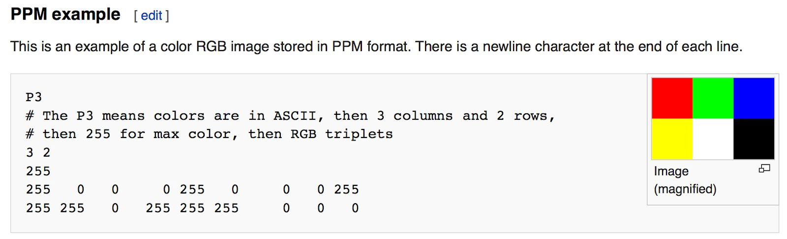
Whenever you start a renderer, you need a way to see an image. The most straightforward way is to write it to a file. The catch is, there are so many formats. Many of those are complex. I always start with a plain text ppm file. Here’s a nice description from Wikipedia:

当你开始写渲染器的时候, 你首先得能有办法看到你渲染的图像。最直接了当的方法就行把图像信息写入文件。问题是, 有那么多图片格式, 而且许多格式都挺复杂的。在开始部分, 我常常使用最简单的ppm文件，这里引用Wikipedia上面的简明介绍:

Let’s make some C++ code to output such a thing:

我们来写一下输出这种图片格式的C++代码:

#include <iostream>

int main() {

    // Image

    const int image_width = 256;
    const int image_height = 256;

    // Render

    std::cout << "P3\n" << image_width << ' ' << image_height << "\n255\n";

    for (int j = image_height-1; j >= 0; --j) {
        for (int i = 0; i < image_width; ++i) {
            auto r = double(i) / (image_width-1);
            auto g = double(j) / (image_height-1);
            auto b = 0.25;

            int ir = static_cast<int>(255.999 * r);
            int ig = static_cast<int>(255.999 * g);
            int ib = static_cast<int>(255.999 * b);

            std::cout << ir << ' ' << ig << ' ' << ib << '\n';
        }
    }
}

There are some things to note in that code:

1. The pixels are written out in rows with pixels left to right.
2. The rows are written out from top to bottom.
3. By convention, each of the red/green/blue components range from 0.0 to 1.0. We will relax that later when we internally use high dynamic range, but before output we will tone map to the zero to one range, so this code won’t change.
4. Red goes from fully off (black) to fully on (bright red) from left to right, and green goes from black at the bottom to fully on at the top. Red and green together make yellow so we should expect the upper right corner to be yellow.

代码里有一些我们要注意的事情:

1. 对于像素来说, 每一行是从左往右写入的。

2. 行从上开始往下写入的。

3. 通常我们把RGB通道的值限定在0.0到1.0。我们之后计算颜色值的时候将使用一个动态的范围, 这个范围并不是0到1。但是在使用这段代码输出图像之前, 我们将把颜色映射到0到1。所以这部分输出图像代码不会改变。

4. 下方的红色从左到右由黑边红, 左侧的绿色从上到下由黑到绿。红+绿变黄, 所以我们的右上角应该是黄的。

下面是我个人的总结，这里有几个之前不是很清楚的点：

• auto关键字就是变量的自动类型推断，可以在声明变量的时候根据变量初始值的类型自动为此变量选择匹配的类型，类似的关键字还有decltype

• static_cast相当于传统的C语言里的强制转换，该运算符把expression转换为new_type类型，用来强迫隐式转换，例如non-const对象转为const对象，编译时检查，用于非多态的转换，可以转换指针及其他，但没有运行时类型检查来保证转换的安全性。它主要有如下几种用法：

  1. 用于类层次结构中基类（父类）和派生类（子类）之间指针或引用的转换

     进行上行转换（把派生类的指针或引用转换成基类表示）是安全的

     进行下行转换（把基类指针或引用转换成派生类表示）时，由于没有动态类型检查，所以是不安全的

  2. 用于基本数据类型之间的转换，如把int转换成char，把int转换成enum。这种转换的安全性也要开发人员来保证

  3. 把空指针转换成目标类型的空指针

  4. 把任何类型的表达式转换成void类型

  注意：static_cast不能转换掉expression的const、volatile、或者__unaligned属性

• 这里行列的变化令人费解，第一层循环负责image_height也就是行的话显然是自顶向上的写入，而文中却说"The rows are written out from top to bottom."，让我感到困惑，可能是为了特定的色彩而故意为之吧

创建图像文件

Because the file is written to the program output, you'll need to redirect it to an image file. Typically this is done from the command-line by using the > redirection operator, like so:

现在我们要把cout的输出流写入文件中。幸好我们有命令行操作符>来定向输出流。在windows操作系统中差不多这样的:

build\Release\inOneWeekend.exe > image.ppm

This is how things would look on Windows. On Mac or Linux, it would look like this:

在Mac或者Linux操作系统中, 大概是这个样子的:

build/inOneWeekend > image.ppm

这里我尝试直接按照上面的代码运行，结果并没有找到build指令。所以我按照linux平台的编译cpp程序的方式，得到了ppm格式的图像：

 g++ -o OneWeekend main.cpp
 ./OneWeekend > image.ppm

Opening the output file (in ToyViewer on my Mac, but try it in your favorite viewer and Google “ppm viewer” if your viewer doesn’t support it) shows this result:

打开我们输出的文件（我是Mac系统, 我是用ToyViewer打开的, 你可以用你喜欢的任意看图软件来打开。如果你默认的看图软件比如windows下的图片不支持ppm格式, 只要Google一下”ppm viewer”装个新的就行。)打开后的结果如下:

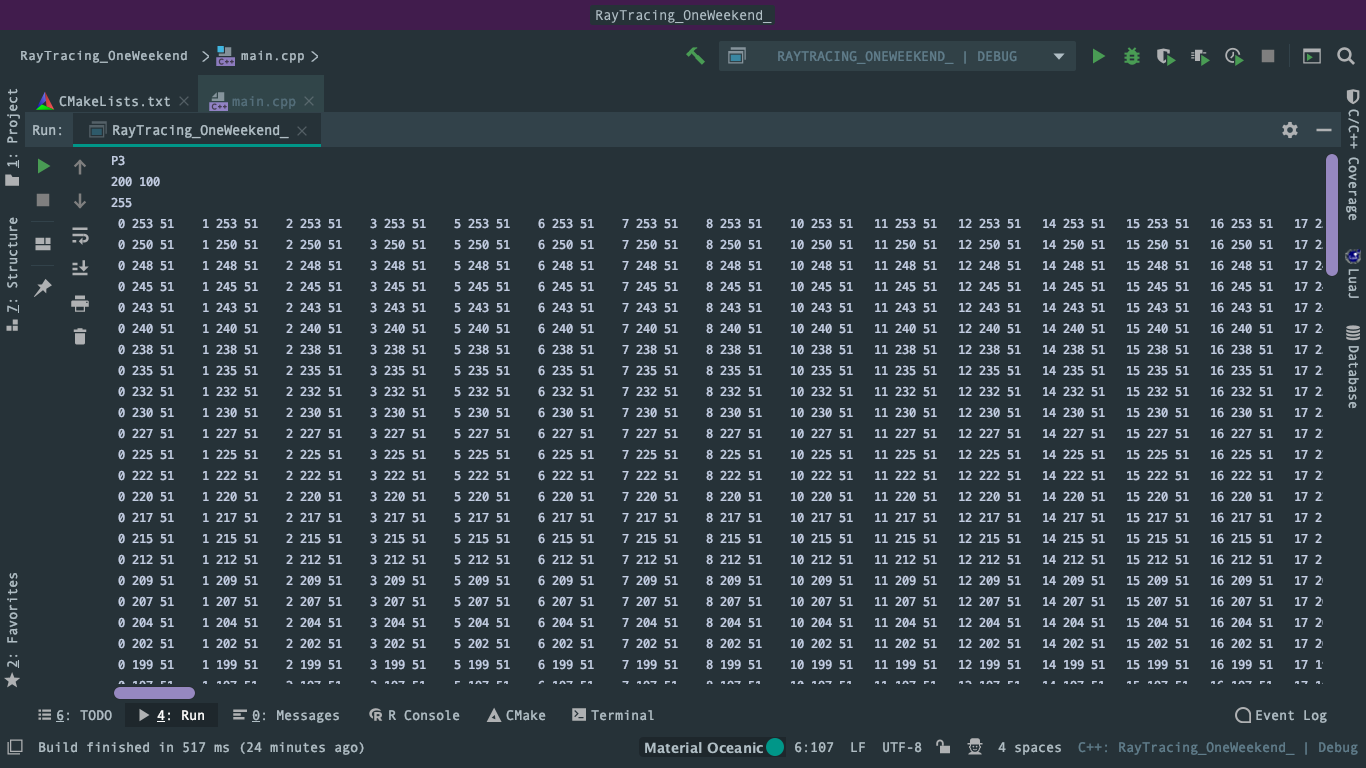
Hooray! This is the graphics “hello world”. If your image doesn’t look like that, open the output file in a text editor and see what it looks like. It should start something like this:

好耶!这便是图形学中的”hello world”了。如果你的图像看上去不是这样的, 用文本编辑器打开你的输出文件, 看看里面内容是啥样的。不出意外的话, 正确格式应该是这样的:

P3
256 256
255
0 255 63
1 255 63
2 255 63
3 255 63
4 255 63
5 255 63
6 255 63
7 255 63
8 255 63
9 255 63
...

If it doesn’t, then you probably just have some newlines or something similar that is confusing the image reader.

If you want to produce more image types than PPM, I am a fan of stb_image.h, a header-only image library available on GitHub at https://github.com/nothings/stb.

如果不是这样的, 你可能当中多了些空行或者类似的什么东西, 因此你的看图软件识别不出来。

如果你想生成别的图像格式来代替基础的PPM, 我强烈安利stb_image.h, 你可以免费在github上获取。

这里我自作聪明将main.cpp中的输出进行了更改，在后面造成了很大的错误：

//std::cout << "\nimage width: " << image_width << "    image height: " << image_height << "\n255\n";
std::cout << "P3\n" << image_width << ' ' << image_height << "\n255\n";

如果不按这种格式生成的.ppm打开会出现格式错误，需要格外注意。

加入一个进度条

Before we continue, let's add a progress indicator to our output. This is a handy way to track the progress of a long render, and also to possibly identify a run that's stalled out due to an infinite loop or other problem.

在我们往下走之前, 我们先来加个输出的进度提示。对于查看一次长时间渲染的进度来说, 这不失为一种简便的做法。也可以通过这个进度来判断程序是否卡住或者进入一个死循环。

Our program outputs the image to the standard output stream (std::cout), so leave that alone and instead write to the error output stream (std::cerr):

我们的程序将图片信息写入标准输出流（std::cout）, 所以我们不能用这个流输出进度。我们换用错误输出流（std::cerr）来输出进度:

    for (int j = image_height-1; j >= 0; --j) {
+       std::cerr << "\rScanlines remaining: " << j << ' ' << std::flush;
        for (int i = 0; i < image_width; ++i) {
            auto r = double(i) / (image_width-1);
            auto g = double(j) / (image_height-1);
            auto b = 0.25;

            int ir = static_cast<int>(255.999 * r);
            int ig = static_cast<int>(255.999 * g);
            int ib = static_cast<int>(255.999 * b);

            std::cout << ir << ' ' << ig << ' ' << ib << '\n';
        }
    }

+  	std::cerr << "\nDone.\n";

vec3向量类

Almost all graphics programs have some class(es) for storing geometric vectors and colors. In many systems these vectors are 4D (3D plus a homogeneous coordinate for geometry, and RGB plus an alpha transparency channel for colors). For our purposes, three coordinates suffices. We’ll use the same class vec3 for colors, locations, directions, offsets, whatever. Some people don’t like this because it doesn’t prevent you from doing something silly, like adding a color to a location. They have a good point, but we’re going to always take the “less code” route when not obviously wrong. In spite of this, we do declare two aliases for vec3: point3 and color. Since these two types are just aliases for vec3, you won't get warnings if you pass a color to a function expecting a point3, for example. We use them only to clarify intent and use.

几乎所有的图形程序都使用类似的类来储存几何向量和颜色。在许多程序中这些向量是四维的(对于位置或者几何向量来说是三维的齐次拓展, 对于颜色来说是RGB加透明通道)。对我们现在这个程序来说, 三维就足够了。我们用一个vec3类来储存所有的颜色, 位置, 方向, 位置偏移, 或者别的什么东西。一些人可能不太喜欢这样做, 因为全都用一个类, 没有限制, 写代码的时候难免会犯二, 比如你把颜色和位置加在一起。他们的想法挺好的, 但是我们想在避免明显错误的同时让代码量尽量的精简。所以这里就先一个类吧。【译注: 之后有添加新的color类】

变量和函数

Here’s the top part of my vec3 class:

下面是我的vec3的头文件:

#ifndef VEC3_H
#define VEC3_H

#include <cmath>
#include <iostream>

using std::sqrt;

class vec3 {
    public:
        vec3() : e{0,0,0} {}
        vec3(double e0, double e1, double e2) : e{e0, e1, e2} {}

        double x() const { return e[0]; }
        double y() const { return e[1]; }
        double z() const { return e[2]; }

        vec3 operator-() const { return vec3(-e[0], -e[1], -e[2]); }
        double operator[](int i) const { return e[i]; }
        double& operator[](int i) { return e[i]; }

        vec3& operator+=(const vec3 &v) {
            e[0] += v.e[0];
            e[1] += v.e[1];
            e[2] += v.e[2];
            return *this;
        }

        vec3& operator*=(const double t) {
            e[0] *= t;
            e[1] *= t;
            e[2] *= t;
            return *this;
        }

        vec3& operator/=(const double t) {
            return *this *= 1/t;
        }

        double length() const {
            return sqrt(length_squared());
        }

        double length_squared() const {
            return e[0]*e[0] + e[1]*e[1] + e[2]*e[2];
        }

    public:
        double e[3];
};

// Type aliases for vec3
using point3 = vec3;   // 3D point
using color = vec3;    // RGB color

#endif

We use double here, but some ray tracers use float. Either one is fine — follow your own tastes.

我们使用双精度浮点double, 但是有些光线追踪器使用单精度浮点float。这里其实都行, 你喜欢哪个就用那个。

vec3实用函数

The second part of the header file contains vector utility functions:

头文件的第二部分包括一些向量操作工具函数:

// vec3 Utility Functions

inline std::ostream& operator<<(std::ostream &out, const vec3 &v) {
    return out << v.e[0] << ' ' << v.e[1] << ' ' << v.e[2];
}

inline vec3 operator+(const vec3 &u, const vec3 &v) {
    return vec3(u.e[0] + v.e[0], u.e[1] + v.e[1], u.e[2] + v.e[2]);
}

inline vec3 operator-(const vec3 &u, const vec3 &v) {
    return vec3(u.e[0] - v.e[0], u.e[1] - v.e[1], u.e[2] - v.e[2]);
}

inline vec3 operator*(const vec3 &u, const vec3 &v) {
    return vec3(u.e[0] * v.e[0], u.e[1] * v.e[1], u.e[2] * v.e[2]);
}

inline vec3 operator*(double t, const vec3 &v) {
    return vec3(t*v.e[0], t*v.e[1], t*v.e[2]);
}

inline vec3 operator*(const vec3 &v, double t) {
    return t * v;
}

inline vec3 operator/(vec3 v, double t) {
    return (1/t) * v;
}

inline double dot(const vec3 &u, const vec3 &v) {
    return u.e[0] * v.e[0]
         + u.e[1] * v.e[1]
         + u.e[2] * v.e[2];
}

inline vec3 cross(const vec3 &u, const vec3 &v) {
    return vec3(u.e[1] * v.e[2] - u.e[2] * v.e[1],
                u.e[2] * v.e[0] - u.e[0] * v.e[2],
                u.e[0] * v.e[1] - u.e[1] * v.e[0]);
}

inline vec3 unit_vector(vec3 v) {
    return v / v.length();
}

光线, 简单摄像机, 以及背景

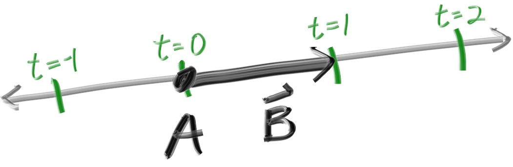
The one thing that all ray tracers have is a ray class and a computation of what color is seen along a ray. Let’s think of a ray as a function P(𝑡)=A+𝑡b. Here P is a 3D position along a line in 3D. A is the ray origin and b is the ray direction. The ray parameter 𝑡t is a real number (double in the code). Plug in a different 𝑡t and P(𝑡) moves the point along the ray. Add in negative 𝑡t values and you can go anywhere on the 3D line. For positive 𝑡t, you get only the parts in front of A, and this is what is often called a half-line or ray.

所有的光线追踪器都有个一个ray类, 我们假定光线的公式为P(𝑡)=A+𝑡b。这里的P是三维射线上的一个点。A是射线的原点, b是射线的方向。类中的变量𝑡是一个实数(代码中为double类型)。P(𝑡)接受任意的𝑡做为变量, 返回射线上的对应点。如果允许𝑡取负值你可以得到整条直线。对于一个正数𝑡, 你只能得到原点前部分A, 这常常被称为半条直线, 或者说射线。

The function P(𝑡) in more verbose code form I call ray::at(t):

我在代码中使用复杂命名, 将函数P(𝑡)扩写为ray::at(t)：

#ifndef RAY_H
#define RAY_H

#include "vec3.h"

class ray {
    public:
        ray() {}
        ray(const vec3& origin, const vec3& direction)
            : orig(origin), dir(direction)
        {}

        vec3 origin() const    { return orig; }
        vec3 direction() const { return dir; }

        vec3 at(double t) const {
            return orig + t*dir;
        }

    public:
        vec3 orig;
        vec3 dir;
};

#endif

Now we are ready to turn the corner and make a ray tracer. At the core, the ray tracer sends rays through pixels and computes the color seen in the direction of those rays. The involved steps are (1) calculate the ray from the eye to the pixel, (2) determine which objects the ray intersects, and (3) compute a color for that intersection point. When first developing a ray tracer, I always do a simple camera for getting the code up and running. I also make a simple ray_color(ray) function that returns the color of the background (a simple gradient).

现在我们再拐回来做我们的光线追踪器。光线追踪器的核心是从像素发射射线, 并计算这些射线得到的颜色。这包括如下的步骤: (1)将射线从视点转化为像素坐标 (2)计算光线是否与场景中的物体相交 (3)如果有, 计算交点的颜色。在做光线追踪器的初期, 我会先弄个简单摄像机让代码能跑起来。我也会编写一个简单的color(ray)函数来返回背景颜色值(一个简单的渐变色)。

I’ve often gotten into trouble using square images for debugging because I transpose 𝑥x and 𝑦y too often, so I’ll use a non-square image. For now we'll use a 16:9 aspect ratio, since that's so common.

在使用正方形的图像Debug时我时常会遇到问题, 因为我老是把x和y弄反。所以我坚持使用16:9这样长宽不等的图像。

In addition to setting up the pixel dimensions for the rendered image, we also need to set up a virtual viewport through which to pass our scene rays. For the standard square pixel spacing, the viewport's aspect ratio should be the same as our rendered image. We'll just pick a viewport two units in height. We'll also set the distance between the projection plane and the projection point to be one unit. This is referred to as the “focal length”, not to be confused with “focus distance”, which we'll present later.

I’ll put the “eye” (or camera center if you think of a camera) at (0,0,0)(0,0,0). I will have the y-axis go up, and the x-axis to the right. In order to respect the convention of a right handed coordinate system, into the screen is the negative z-axis. I will traverse the screen from the upper left hand corner, and use two offset vectors along the screen sides to move the ray endpoint across the screen. Note that I do not make the ray direction a unit length vector because I think not doing that makes for simpler and slightly faster code.

我会把视点(或者说摄像机, 如果你认为它是个摄像机的话)放在(0,0,0)(0,0,0)。这里y轴向上, x轴向右, 为了准守使用左手系的规范, 摄像机看向的方向为z轴的负方向。我会把发出射线的原点从图像的左下角开始沿着xy方向做增量直至遍历全图。注意我这里并没有将射线的向量设置为单位向量, 因为我认为这样代码会更加简单快捷。

Below in code, the ray r goes to approximately the pixel centers (I won’t worry about exactness for now because we’ll add antialiasing later):

下面是代码, 射线r现在只是近似的从各个像素的中心射出(现在不必担心精度问题, 因为我们一会儿就会加入抗锯齿):

#include "vec3.h"

#include <iostream>

int main() {
    const int image_width = 200;
    const int image_height = 100;

    std::cout << "P3\n" << image_width << ' ' << image_height << "\n255\n";

    for (int j = image_height-1; j >= 0; --j) {
        std::cerr << "\rScanlines remaining: " << j << ' ' << std::flush;
        for (int i = 0; i < image_width; ++i) {
+            vec3 color(double(i)/image_width, double(j)/image_height, 0.2);
+            color.write_color(std::cout);
        }
    }

    std::cerr << "\nDone.\n";
}

The ray_color(ray) function linearly blends white and blue depending on the height of the 𝑦 coordinate after scaling the ray direction to unit length (so $−1.0<𝑦<1.0$). Because we're looking at the 𝑦 height after normalizing the vector, you'll notice a horizontal gradient to the color in addition to the vertical gradient.

I then did a standard graphics trick of scaling that to $0.0≤𝑡≤1.0$. When $𝑡=1.0$ I want blue. When $𝑡=0.0$ I want white. In between, I want a blend. This forms a “linear blend”, or “linear interpolation”, or “lerp” for short, between two things. A lerp is always of the form

ray_color(ray)函数根据y值将蓝白做了个线性差值的混合, 我们这里把射线做了个单位化, 以保证y的取值范围($−1.0<y<1.0$)。因为我们使用y轴做渐变, 所以你可以看到这个蓝白渐变也是竖直的。

我接下来使用了一个标准的小技巧将y的范围从$−1.0≤y≤1.0$映射到了$0≤y≤1.0$。这样$t=1.0$时就是蓝色, 而$t=0.0$时就是白色。在蓝白之间我想要一个混合效果(blend)。现在我们采用的是线性混合(linear blend)或者说线性插值(liner interpolation)。或者简称其为lerp。一个lerp一般来说会是下面的形式: $$ blendedValue=(1−t)⋅startValue+t⋅endValue $$

with 𝑡 going from zero to one. In our case this produces:

当$t$从0到1, 我们会渲染出这样的图像:

加入球体

Let’s add a single object to our ray tracer. People often use spheres in ray tracers because calculating whether a ray hits a sphere is pretty straightforward.

让我们为我们的光线追踪器加入一个物体吧!人们通常使用的球体, 因为计算射线是否与球体相交是十分简洁明了的。

Recall that the equation for a sphere centered at the origin of radius 𝑅R is $x^2+y^2+z^2=R^2$. Put another way, if a given point $(𝑥,𝑦,𝑧)$ is on the sphere, then $x^2+y^2+z^2=R^2$. If the given point (𝑥,𝑦,𝑧)(x,y,z) is inside the sphere, then $x^2+y^2+z^2<R^2$, and if a given point$ (𝑥,𝑦,𝑧)$ is outside the sphere, then $x^2+y^2+z^2>R^2$.

It gets uglier if the sphere center is at (𝐶𝑥,𝐶𝑦,𝐶𝑧):

回想一下我们中学时期学过的球体表面方程, 对于一个半径为r的球体来说, 有方程$x^2+y^2+z^2=R^2$, 其中$(x,y,z)$是球面上的点。如果我们想要表示点$(x,y,z)$在球体的内部, 那便有方程$x^2+y^2+z^2<R^2$, 类似的, 如果要表示球体外部的点, 则有$x^2+y^2+z^2>R^2$。

如果球体的球心在$(c_x,c_y,c_z)$, 那么这个式子就会变得丑陋一些: $$ (x−c_x)2+(y−c_y)^2+(z−c_z)^2=R^2 $$

在图形学中, 你总希望你方程里面所有东西都是用向量表达的, 这样我们就能用vec3这个类来存储所有的这些xyz相关的东西了。你也许会意识到, 对于到球面上的点$P=(x,y,z)$到球心$c=(c_x,c_y,c_z)$的距离可以使用向量表示为$(p−c)$, 于是就有 $$ (p−c)⋅(p−c)=(x−c_x)2+(y−c_y)2+(z−c_z)2 $$

So the equation of the sphere in vector form is:

于是我们就能得到球面方程的向量形式: $$ (p−c)⋅(p−c)=R^2 $$

We can read this as “any point 𝐏 that satisfies this equation is on the sphere”. We want to know if our ray $P(t)=A+tb$ ever hits the sphere anywhere. If it does hit the sphere, there is some 𝑡t for which $P(t) $satisfies the sphere equation. So we are looking for any 𝑡t where this is true:

我们可以将其解读为”满足方程上述方程的任意一点$p$一定位于球面上”。我们还要知道射线$p(t)=a+t \vec b$是否与球体相交。如果说它相交了, 那么肯定有一个$t$使直线上的点$p(t)$满足球面方程。所以我们先来计算满足条件的任意$t$值: $$ (p(t)−c)⋅(p(t)−c)=R^2 $$

or expanding the full form of the ray $P(t)$:

或者将$p(t)$展开为射线方程: $$ (a+t \vec b−c)⋅(a+t \vec b−c)=R^2 $$

The rules of vector algebra are all that we would want here. If we expand that equation and move all the terms to the left hand side we get:

好啦, 我们需要的代数部分就到这里。现在我们来展开表达式并移项, 得: $$ t^2 \vec b⋅\vec b+2t \vec b⋅\vec{(a−c)}+ \vec{(a−c)}⋅\vec {(a−c)}−R^2=0 $$

The vectors and 𝑟r in that equation are all constant and known. The unknown is 𝑡, and the equation is a quadratic, like you probably saw in your high school math class. You can solve for 𝑡t and there is a square root part that is either positive (meaning two real solutions), negative (meaning no real solutions), or zero (meaning one real solution). In graphics, the algebra almost always relates very directly to the geometry. What we have is:

方程中的向量和半径R都是已知的常量, 唯一的未知数就是t, 并且这个等式是关于t的一个一元二次方程, 就像你在高中数学课上【？？？】学到的那样。你可以用求根公式来判别交点个数, 为正则2个交点, 为负则1个交点, 为0则没有交点。在图形学中, 代数与几何往往密切相关, 你看图:

If we take that math and hard-code it into our program, we can test it by coloring red any pixel that hits a small sphere we place at −1 on the z-axis:

如果我们使用代码来求解, 并使用红色来表示射线击中我们放在$(0,0,-1)$的小球:

bool hit_sphere(const vec3& center, double radius, const ray& r) {
    vec3 oc = r.origin() - center;
    auto a = dot(r.direction(), r.direction());
    auto b = 2.0 * dot(oc, r.direction());
    auto c = dot(oc, oc) - radius*radius;
    auto discriminant = b*b - 4*a*c;
    return (discriminant > 0);
}

+vec3 ray_color(const ray& r) {
+    if (hit_sphere(vec3(0,0,-1), 0.5, r))
+        return vec3(1, 0, 0);
    vec3 unit_direction = unit_vector(r.direction());
    auto t = 0.5*(unit_direction.y() + 1.0);
    return (1.0-t)*vec3(1.0, 1.0, 1.0) + t*vec3(0.5, 0.7, 1.0);
}

我们会得到:

现在我们啥都缺: 例如光照, 反射, 加入更多的物体, 但是我们离成功又近了一步!现在你要注意我们其实求的是直线与球相交的解, $t&lt;0$的那些情况也计算进去了, 而我们只想要直线中一段射线的解。如果你将你的球心设置在$(0,0,1)$你会得到完全相同的结果。这不是一个特性(feature)!【吐槽: 直接说it’s a bug嘛】我们会在接下来的章节修复这个bug。

面法线与复数物体

First, let’s get ourselves a surface normal so we can shade. This is a vector that is perpendicular to the surface at the point of intersection. There are two design decisions to make for normals. The first is whether these normals are unit length. That is convenient for shading so I will say yes, but I won’t enforce that in the code. This could allow subtle bugs, so be aware this is personal preference as are most design decisions like that. For a sphere, the outward normal is in the direction of the hit point minus the center:

为了来给球体着色, 首先我们来定义一下面法线。面法线应该是一种垂直于交点所在平面的三维向量。关于面法线我们存在两个设计抉择。首先是是否将其设计为单位向量, 这样对于着色器来说, 所以我会说”yes!”但是我并没有在代码里这么做, 这部分差异可能会导致一些潜在的bug。所以记住, 这个是个人喜好, 大多数的人喜好使用单位法线。对于球体来说, 朝外的法线是直线与球的交点减去球心:

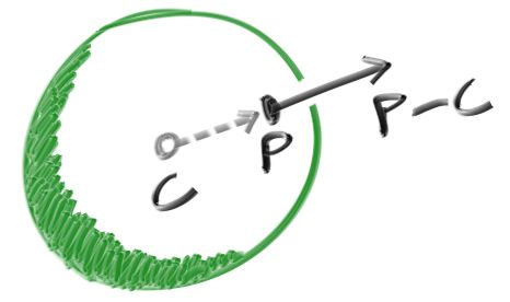
On the earth, this implies that the vector from the earth’s center to you points straight up. Let’s throw that into the code now, and shade it. We don’t have any lights or anything yet, so let’s just visualize the normals with a color map. A common trick used for visualizing normals (because it’s easy and somewhat intuitive to assume 𝐧 is a unit length vector — so each component is between −1 and 1) is to map each component to the interval from 0 to 1, and then map x/y/z to r/g/b. For the normal, we need the hit point, not just whether we hit or not. We only have one sphere in the scene, and it's directly in front of the camera, so we won't worry about negative values of 𝑡t yet. We'll just assume the closest hit point (smallest 𝑡t). These changes in the code let us compute and visualize 𝐧:

说到底, 其实就是从球心到交点再向外延伸的那个方向。让我们把这部分转变成代码并开始着色。我们暂时还没有光源这样的东西, 所以让我们直接将法线值作为颜色输出吧。对于法线可视化来说, 我们常常将xyz分量的值先映射到0到1的范围(假定vecN是一个单位向量, 它的取值范围是-1到1的),再把它赋值给rgb。对于法线来说, 光能判断射线是否与球体相交是不够的, 我们还需求出交点的坐标。在有两个交点的情况下, 我们选取最近的交点smallest(t)。计算与可视化球的法向量的代码如下:

+double hit_sphere(const vec3& center, double radius, const ray& r) {
    vec3 oc = r.origin() - center;
    auto a = dot(r.direction(), r.direction());
    auto b = 2.0 * dot(oc, r.direction());
    auto c = dot(oc, oc) - radius*radius;
    auto discriminant = b*b - 4*a*c;
+    if (discriminant < 0) {
+        return -1.0;
+    } else {
+        return (-b - sqrt(discriminant) ) / (2.0*a);
+    }
}

vec3 ray_color(const ray& r) {
+    auto t = hit_sphere(vec3(0,0,-1), 0.5, r);
+    if (t > 0.0) {
+        vec3 N = unit_vector(r.at(t) - vec3(0,0,-1));
+        return 0.5*vec3(N.x()+1, N.y()+1, N.z()+1);
+    }
    vec3 unit_direction = unit_vector(r.direction());
+    t = 0.5*(unit_direction.y() + 1.0);
    return (1.0-t)*vec3(1.0, 1.0, 1.0) + t*vec3(0.5, 0.7, 1.0);
}

这会得到下面的结果:

还有一种基于计算过程对代码的简化，我也写出来供参考，但这个简化效率提升不多，所以代码保留之前好理解的。

Let’s revisit the ray-sphere equation:

我们再来回顾上面的直线方程:

vec3 oc = r.origin() - center;
auto a = dot(r.direction(), r.direction());
auto b = 2.0 * dot(oc, r.direction());
auto c = dot(oc, oc) - radius*radius;
auto discriminant = b*b - 4*a*c;

First, recall that a vector dotted with itself is equal to the squared length of that vector.

Second, notice how the equation for b has a factor of two in it. Consider what happens to the quadratic equation if 𝑏=2ℎ:

首先, 回想一下一个向量与自己的点积就是它的长度的平方(都是$x^2+y^2+z^2$)

其次, 注意其实我们的b有一个系数2, 我们设b=2h, 有:

$\frac{-b +/- \sqrt{b^2-4ac}}{2a} = \frac{-2h +/- \sqrt{(2h)^2-4ac}}{2a} = \frac{-h +/- \sqrt{h^2-ac}}{a}$

Using these observations, we can now simplify the sphere-intersection code to this:

所以射线与球体求交的代码其实可以简化成下面这样:

vec3 oc = r.origin() - center;
-auto a = dot(r.direction(), r.direction());
-auto b = 2.0 * dot(oc, r.direction());
-auto c = dot(oc, oc) - radius*radius;
-auto discriminant = b*b - 4*a*c;
+auto a = r.direction().length_squared();
+auto half_b = dot(oc, r.direction());
+auto c = oc.length_squared() - radius*radius;
+auto discriminant = half_b*half_b - a*c;

if (discriminant < 0) {
    return -1.0;
} else {
-   return (-b - sqrt(discriminant) ) / (2.0*a);
+   return (-half_b - sqrt(discriminant) ) / a;
}

Now, how about several spheres? While it is tempting to have an array of spheres, a very clean solution is the make an “abstract class” for anything a ray might hit, and make both a sphere and a list of spheres just something you can hit. What that class should be called is something of a quandary — calling it an “object” would be good if not for “object oriented” programming. “Surface” is often used, with the weakness being maybe we will want volumes. “hittable” emphasizes the member function that unites them. I don’t love any of these, but I will go with “hittable”.

好啦, 那么怎么在场景中渲染不止一个球呢? 很直接的我们想到使用一个sphere数组, 这里有个很简洁的好方法: 使用一个抽象类, 任何可能与光线求交的东西实现时都继承这个类, 并且让球以及球列表也都继承这个类。我们该给这个类起个什么样的名字呢? 叫它object好像不错但现在我们使用面向对象编程(oop)。suface是时常被翻牌, 但是如果我们想要体积体(volumes)的话就不太适合了。hittable又过于强调了自己的成员函数hit。所以我哪个都不喜欢, 但是总得给它个名字的嘛, 那我就叫它hittable。

This hittable abstract class will have a hit function that takes in a ray. Most ray tracers have found it convenient to add a valid interval for hits 𝑡𝑚𝑖𝑛tmin to 𝑡𝑚𝑎𝑥tmax, so the hit only “counts” if $𝑡_{𝑚𝑖𝑛}&lt;𝑡&lt;𝑡_{𝑚𝑎𝑥}$. For the initial rays this is positive 𝑡t, but as we will see, it can help some details in the code to have an interval $𝑡_{𝑚𝑖𝑛}$ to $𝑡_{𝑚𝑎𝑥}$. One design question is whether to do things like compute the normal if we hit something. We might end up hitting something closer as we do our search, and we will only need the normal of the closest thing. I will go with the simple solution and compute a bundle of stuff I will store in some structure. Here’s the abstract class:

hittable类理应有个接受射线为参数的函数, 许多光线追踪器为了便利, 加入了一个区间$t_{min}<t<t_{max}$来判断相交是否有效。对于一开始的光线来说, 这个t值总是正的, 但加入这部分对代码实现的一些细节有着不错的帮助。现在有个设计上的问题:我们是否在每次计算求交的时候都要去计算法相?但其实我们只需要计算离射线原点最近的那个交点的法相就行了, 后面的东西会被遮挡。接下来我会给出我的代码, 并将一些计算的结果存在一个结构体里, 来看, 这就是那个抽象类:

#ifndef HITTABLE_H
#define HITTABLE_H

#include "ray.h"

struct hit_record {
    vec3 p;
    vec3 normal;
    double t;
};

class hittable {
    public:
        virtual bool hit(const ray& r, double t_min, double t_max, hit_record& rec) const = 0;
};

#endif

And here’s the sphere:

#ifndef SPHERE_H
#define SPHERE_H

#include "hittable.h"
#include "vec3.h"

class sphere: public hittable {
    public:
        sphere() {}
        sphere(vec3 cen, double r) : center(cen), radius(r) {};

        virtual bool hit(const ray& r, double tmin, double tmax, hit_record& rec) const;

    public:
        vec3 center;
        double radius;
};

bool sphere::hit(const ray& r, double t_min, double t_max, hit_record& rec) const {
    vec3 oc = r.origin() - center;
    auto a = r.direction().length_squared();
    auto half_b = dot(oc, r.direction());
    auto c = oc.length_squared() - radius*radius;
    auto discriminant = half_b*half_b - a*c;

    if (discriminant > 0) {
        auto root = sqrt(discriminant);
        auto temp = (-half_b - root)/a;
        if (temp < t_max && temp > t_min) {
            rec.t = temp;
            rec.p = r.at(rec.t);
            rec.normal = (rec.p - center) / radius;
            return true;
        }
        temp = (-half_b + root) / a;
        if (temp < t_max && temp > t_min) {
            rec.t = temp;
            rec.p = r.at(rec.t);
            rec.normal = (rec.p - center) / radius;
            return true;
        }
    }
    return false;
}


#endif

The second design decision for normals is whether they should always point out. At present, the normal found will always be in the direction of the center to the intersection point (the normal points out). If the ray intersects the sphere from the outside, the normal points against the ray. If the ray intersects the sphere from the inside, the normal (which always points out) points with the ray. Alternatively, we can have the normal always point against the ray. If the ray is outside the sphere, the normal will point outward, but if the ray is inside the sphere, the normal will point inward.

好了, 让我们来谈谈第二个关于面法相设计上的问题吧， 那就是面法相的朝向问题。对于现在来说, 如果光线从球体外部击中球体, 那么法相也是朝外的, 与射线的方向相反(不是数学意义上的严格相反, 只是大致逆着)。如果光线从内部射向球面时, 此时的面法相依然朝外, 与射线方向相同。相对的, 我们也可以总是让法相向量与射线方向相反, 即射线从外部射向球面, 法向量朝外, 射线从内部射向球面, 法向量向着球心。

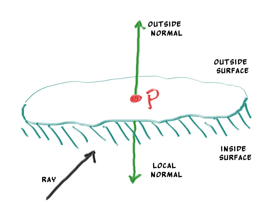
We need to choose one of these possibilities because we will eventually want to determine which side of the surface that the ray is coming from. This is important for objects that are rendered differently on each side, like the text on a two-sided sheet of paper, or for objects that have an inside and an outside, like glass balls.

在我们着色前, 我们需要仔细考虑一下采用上面哪种方式, 这对于双面材质来说至关重要。例如一张双面打印的A4纸, 或者玻璃球这样的同时具有内表面和外表面的物体。

If we decide to have the normals always point out, then we will need to determine which side the ray is on when we color it. We can figure this out by comparing the ray with the normal. If the ray and the normal face in the same direction, the ray is inside the object, if the ray and the normal face in the opposite direction, then the ray is outside the object. This can be determined by taking the dot product of the two vectors, where if their dot is positive, the ray is inside the sphere.

如果我们决定让法相永远朝外, 那在我们就得在射入的时候判断是从表面的哪一侧射入的, 我们可以简单的将光线与法相做点乘来判断。如果法相与光线方向相同, 那就是从内部击中内表面, 如果相反则是从外部击中外表面。【译注: $dot(a,b)=cosθ|a||b|$】

if (dot(ray_direction, outward_normal) > 0.0) {
    // ray is inside the sphere
    ...
} else {
    // ray is outside the sphere
    ...
}

If we decide to have the normals always point against the ray, we won't be able to use the dot product to determine which side of the surface the ray is on. Instead, we would need to store that information:

如果我们永远让法相与入射方向相反, 我们就不用去用点乘来判断射入面是内侧还是外侧了, 但相对的, 我们需要用一个变量储存摄入面的信息:

bool front_face;
if (dot(ray_direction, outward_normal) > 0.0) {
    // ray is inside the sphere
    normal = -outward_normal;
    front_face = false;
}
else {
    // ray is outside the sphere
    normal = outward_normal;
    front_face = true;
}

We can set things up so that normals always point “outward” from the surface, or always point against the incident ray. This decision is determined by whether you want to determine the side of the surface at the time of geometry intersection or at the time of coloring. In this book we have more material types than we have geometry types, so we'll go for less work and put the determination at geometry time. This is simply a matter of preference, and you'll see both implementations in the literature.

We add the front_face bool to the hit_record struct. We'll also add a function to solve this calculation for us.

其实采取哪种策略, 关键在于你想把这部分放在着色阶段还是几何求交的阶段。【译注:反正都要算的, v2.0的时候是在着色阶段判别的, v3.0把它放在了求交阶段】。在本书中我们我们的材质类型会比我们的几何图元类型多, 所以为了有更少的代码量, 我们会在几何部分先判别射入面是内侧还是外侧。这当然也是一种个人喜好。

我们在结构体hit_record中加入front_face变量, 我们接下来还会弄一些动态模糊相关的事情(Book2 chapter1),所以我还会加入一个时间变量:

ifndef HITTABLE_H
#define HITTABLE_H

#include "ray.h"

struct hit_record {
    vec3 p;
    vec3 normal;
+    double t;
+    bool front_face;

+    inline void set_face_normal(const ray& r, const vec3& outward_normal) {
        front_face = dot(r.direction(), outward_normal) < 0;
        normal = front_face ? outward_normal :-outward_normal;
    }
};

class hittable {
    public:
        virtual bool hit(const ray& r, double t_min, double t_max, hit_record& rec) const = 0;
};
#endif

And then we add the surface side determination to the class:

接下来我们在求交时加入射入面的判别:

bool sphere::hit(const ray& r, double t_min, double t_max, hit_record& rec) const {
    vec3 oc = r.origin() - center;
    auto a = r.direction().length_squared();
    auto half_b = dot(oc, r.direction());
    auto c = oc.length_squared() - radius*radius;
    auto discriminant = half_b*half_b - a*c;

    if (discriminant > 0) {
        auto root = sqrt(discriminant);
        auto temp = (-half_b - root)/a;
        if (temp < t_max && temp > t_min) {
            rec.t = temp;
            rec.p = r.at(rec.t);
+            vec3 outward_normal = (rec.p - center) / radius;
+            rec.set_face_normal(r, outward_normal);
            return true;
        }
        temp = (-half_b + root) / a;
        if (temp < t_max && temp > t_min) {
            rec.t = temp;
            rec.p = r.at(rec.t);
+            vec3 outward_normal = (rec.p - center) / radius;
+            rec.set_face_normal(r, outward_normal);
            return true;
        }
    }
    return false;
}

我们加入存放物体的列表：

#ifndef HITTABLE_LIST_H
#define HITTABLE_LIST_H

#include "hittable.h"
#include <memory>
#include <vector>

using std::shared_ptr;
using std::make_shared;

class hittable_list: public hittable {
    public:
        hittable_list() {}
        hittable_list(shared_ptr<hittable> object) { add(object); }

        void clear() { objects.clear(); }
        void add(shared_ptr<hittable> object) { objects.push_back(object); }

        virtual bool hit(const ray& r, double tmin, double tmax, hit_record& rec) const;

    public:
        std::vector<shared_ptr<hittable>> objects;
};

bool hittable_list::hit(const ray& r, double t_min, double t_max, hit_record& rec) const {
    hit_record temp_rec;
    bool hit_anything = false;
    auto closest_so_far = t_max;

    for (const auto& object : objects) {
        if (object->hit(r, t_min, closest_so_far, temp_rec)) {
            hit_anything = true;
            closest_so_far = temp_rec.t;
            rec = temp_rec;
        }
    }

    return hit_anything;
}

#endif

一些C++的新特性

The hittable_list class code uses two C++ features that may trip you up if you're not normally a C++ programmer: vector and shared_ptr.

hittable_list类使用了两种C++的特性:vector和shared_ptr, 如果你并不熟悉C++, 你可能会感到有些困惑。

shared_ptr

shared_ptr<type> is a pointer to some allocated type, with reference-counting semantics. Every time you assign its value to another shared pointer (usually with a simple assignment), the reference count is incremented. As shared pointers go out of scope (like at the end of a block or function), the reference count is decremented. Once the count goes to zero, the object is deleted.

shared_ptr<type>是指向一些已分配内存的类型的指针。每当你将它的值赋值给另一个智能指针时, 物体的引用计数器就会+1。当智能指针离开它所在的生存范围(例如代码块或者函数外), 物体的引用计数器就会-1。一旦引用计数器为0, 即没有任何智能指针指向该物体时, 该物体就会被销毁。

Typically, a shared pointer is first initialized with a newly-allocated object, something like this:

一般来说, 智能指针首先由一个刚刚新分配好内存的物体来初始化:

shared_ptr<double> double_ptr = make_shared<double>(0.37);
shared_ptr<vec3>   vec3_ptr   = make_shared<vec3>(1.414214, 2.718281, 1.618034);
shared_ptr<sphere> sphere_ptr = make_shared<sphere>(vec3(0,0,0), 1.0);

make_shared<thing>(thing_constructor_params ...) allocates a new instance of type thing, using the constructor parameters. It returns a shared_ptr<thing>.

Since the type can be automatically deduced by the return type of make_shared<type>(...), the above lines can be more simply expressed using C++'s auto type specifier:

make_shared<thing>(thing_constructor_params ...)为指定的类型分配一段内存, 使用你指定的构造函数与参数来创建这个类, 并返回一个智能指针shared_ptr<thing>

使用C++的auto类型关键字, 可以自动推断make_shared<type>返回的智能指针类型, 于是我们可以把上面的代码简化为:

auto double_ptr = make_shared<double>(0.37);
auto vec3_ptr   = make_shared<vec3>(1.414214, 2.718281, 1.618034);
auto sphere_ptr = make_shared<sphere>(vec3(0,0,0), 1.0);

We'll use shared pointers in our code, because it allows multiple geometries to share a common instance (for example, a bunch of spheres that all use the same texture map material), and because it makes memory management automatic and easier to reason about.

std::shared_ptr is included with the <memory> header.

我们在代码中使用智能指针的目的是为了能让多个几何图元共享一个实例(举个栗子, 一堆不同球体使用同一个纹理材质), 并且这样内存管理比起普通的指针更加的简单方便。

std::shared_ptr在头文件<memory>中:

#include <memory>

vector

The second C++ feature you may be unfamiliar with is std::vector. This is a generic array-like collection of an arbitrary type. Above, we use a collection of pointers to hittable. std::vector automatically grows as more values are added: objects.push_back(object) adds a value to the end of the std::vector member variable objects.

第二个你可能不太熟悉的C++特性是std::vector。这是一个类似数组的结构类型, 可以存储任意指定的类型。在上面的代码中, 我们将hittable类型的智能指针存入vector中, 随着objects.push_back(object)的调用, object被存入vector的末尾, 同时vector的储存空间会自动增加。

std::vector is included with the <vector> header.

std::vector在头文件<vector>中

#include <vector>

Finally, the using statements in listing 20 tell the compiler that we'll be getting shared_ptr and make_shared from the std library, so we don't need to prefex these with std:: every time we reference them.

最后, 位于hittable_list.h文件开头部分的using语句告诉编译器, shared_ptr与make_shared是来自std库的。这样我们在使用它们之前就不用每次都加上前缀std::。

常用的常数与工具函数

我们需要在头文件中定义一些常用的常数。目前为止我们只需要定义无穷。但是我们先把pi在这里定义好, 之后要用的。对于pi来说并没有什么跨平台的标准定义【译注: 这就是为什么不使用之前版本中M_PI宏定义的原因】, 所以我们自己来定义一下。我们在rtweekend.h中给出了一些未来常用的常数和函数:

#ifndef RTWEEKEND_H
#define RTWEEKEND_H

#include <cmath>
#include <cstdlib>
#include <limits>
#include <memory>


// Usings

using std::shared_ptr;
using std::make_shared;

// Constants

const double infinity = std::numeric_limits<double>::infinity();
const double pi = 3.1415926535897932385;

// Utility Functions

inline double degrees_to_radians(double degrees) {
    return degrees * pi / 180;
}

inline double ffmin(double a, double b) { return a <= b ? a : b; }
inline double ffmax(double a, double b) { return a >= b ? a : b; }

// Common Headers

#include "ray.h"
#include "vec3.h"

#endif

以及这是更新后的main函数:

#include "rtweekend.h"
#include "hittable_list.h"
#include "sphere.h"
#include <iostream>

vec3 ray_color(const ray& r, const hittable& world) {
+    hit_record rec;
+    if (world.hit(r, 0, infinity, rec)) {
+        return 0.5 * (rec.normal + vec3(1,1,1));
+    }    

     vec3 unit_direction = unit_vector(r.direction());
+    auto t = 0.5*(unit_direction.y() + 1.0);    
     return (1.0-t)*vec3(1.0, 1.0, 1.0) + t*vec3(0.5, 0.7, 1.0);
}

int main() {    
    const int image_width = 200;    
    const int image_height = 100;    

    std::cout << "P3\n" << image_width << ' ' << image_height << "\n255\n";    
    vec3 lower_left_corner(-2.0, -1.0, -1.0);    
    vec3 horizontal(4.0, 0.0, 0.0);    
    vec3 vertical(0.0, 2.0, 0.0);    
    vec3 origin(0.0, 0.0, 0.0);
+    hittable_list world;
+    world.add(make_shared<sphere>(vec3(0,0,-1), 0.5));
+    world.add(make_shared<sphere>(vec3(0,-100.5,-1), 100));    
    
    for (int j = image_height-1; j >= 0; --j) {        
        std::cerr << "\rScanlines remaining: " << j << ' ' << std::flush;        
        for (int i = 0; i < image_width; ++i) {            
            auto u = double(i) / image_width;            
            auto v = double(j) / image_height;            
            ray r(origin, lower_left_corner + u*horizontal + v*vertical);
+           vec3 color = ray_color(r, world);            
            color.write_color(std::cout);        
        }    
    }    
    std::cerr << "\nDone.\n";
}

这样我们就会得到一张使用法向作为球体颜色值的图片。当你想查看模型的特征细节与瑕疵时, 输出面法向作为颜色值不失为一种很好的方法。

反走样

When a real camera takes a picture, there are usually no jaggies along edges because the edge pixels are a blend of some foreground and some background. We can get the same effect by averaging a bunch of samples inside each pixel. We will not bother with stratification. This is controversial, but is usual for my programs. For some ray tracers it is critical, but the kind of general one we are writing doesn’t benefit very much from it and it makes the code uglier. We abstract the camera class a bit so we can make a cooler camera later.

真实世界中的摄像机拍摄出来的照片是没有像素状的锯齿的。因为边缘像素是由背景和前景混合而成的。我们也可以在程序中简单的对每个边缘像素多次采样取平均达到类似的效果。我们这里不会使用分层采样。尽管我自己常常在我的程序里使用这种有争议的方法。对某些光线追踪器来说分层采样是很关键的部分, 但是对于我们写的这个小光线追踪器并不会有什么很大的提升, 只会让代码更加丑陋。我们会在这里将摄像机类抽象一下, 以便于后续能有一个更酷的摄像机。

When a real camera takes a picture, there are usually no jaggies along edges because the edge pixels are a blend of some foreground and some background. We can get the same effect by averaging a bunch of samples inside each pixel. We will not bother with stratification. This is controversial, but is usual for my programs. For some ray tracers it is critical, but the kind of general one we are writing doesn’t benefit very much from it and it makes the code uglier. We abstract the camera class a bit so we can make a cooler camera later.

我们还需要一个能够返回真随机数的一个随机数生成器。默认来说这个函数应该返回0≤r<1的随机数。注意这个范围取不到1是很重要的。有时候我们能从这个特性中获得好处。

A simple approach to this is to use the rand() function that can be found in <cstdlib>. This function returns a random integer in the range 0 and RAND_MAX. Hence we can get a real random number as desired with the following code snippet, added to rtweekend.h:

一个简单的实现方法是, 使用<cstdlib>中的rand()函数。这个函数会返回0到RAND_MAX中的一个任意整数。我们将下面的一小段代码加到rtweekend.h中, 就能得到我们想要的随机函数了:

#include <cstdlib>
...

inline double random_double() {
    // Returns a random real in [0,1).
    return rand() / (RAND_MAX + 1.0);
}

inline double random_double(double min, double max) {
    // Returns a random real in [min,max).
    return min + (max-min)*random_double();
}

C++ did not traditionally have a standard random number generator, but newer versions of C++ have addressed this issue with the <random> header (if imperfectly according to some experts). If you want to use this, you can obtain a random number with the conditions we need as follows:

传统C++并没有随机数生成器, 但是新版C++中的头实现了这个功能(某些专家觉得这种方法不太完美)。如果你想使用这种方法, 你可以参照下面的代码:

#include <functional>
#include <random>

inline double random_double() {
    static std::uniform_real_distribution<double> distribution(0.0, 1.0);
    static std::mt19937 generator;
    static std::function<double()> rand_generator =
        std::bind(distribution, generator);
    return rand_generator();
}

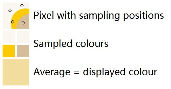
For a given pixel we have several samples within that pixel and send rays through each of the samples. The colors of these rays are then averaged:

对于给定的像素, 我们发射多条射线进行多次采样。然后我们对颜色结果求一个平均值:

Now's a good time to create a camera class to manage our virtual camera and the related tasks of scene scampling. The following class implements a simple camera using the axis-aligned camera from before:

综上, 我们对我们的简单的轴对齐摄像机类进行了一次封装:

#ifndef CAMERA_H
#define CAMERA_H

#include "rtweekend.h"

class camera {
    public:
        camera() {
            lower_left_corner = vec3(-2.0, -1.0, -1.0);
            horizontal = vec3(4.0, 0.0, 0.0);
            vertical = vec3(0.0, 2.0, 0.0);
            origin = vec3(0.0, 0.0, 0.0);
        }

        ray get_ray(double u, double v) {
            return ray(origin, lower_left_corner + u*horizontal + v*vertical - origin);
        }

    public:
        vec3 origin;
        vec3 lower_left_corner;
        vec3 horizontal;
        vec3 vertical;
};
#endif

To handle the multi-sampled color computation, we'll update the write_color() function. Rather than adding in a fractional contribution each time we accumulate more light to the color, just add the full color each iteration, and then perform a single divide at the end (by the number of samples) when writing out the color. In addition, we'll add a handy utility function to the rtweekend.h utility header: clamp(x,min,max), which clamps the value x to the range [min,max]:

为了对多重采样的颜色值进行计算, 我们升级了vec3::write_color()函数。我们不会在每次发出射线采样时都计算一个0-1之间的颜色值, 而是一次性把所有的颜色都加在一起, 然后最后只需要简单的一除(除以采样点个数)。另外, 我们给头文件rtweekend.h加入了一个新函数clamp(x,min,max), 用来将x限制在[min,max]区间之中:

inline double clamp(double x, double min, double max) {
    if (x < min) return min;
    if (x > max) return max;
    return x;
}

void write_color(std::ostream &out, int samples_per_pixel) {
    // Divide the color total by the number of samples.
    auto scale = 1.0 / samples_per_pixel;
    auto r = scale * e[0];
    auto g = scale * e[1];
    auto b = scale * e[2];

    // Write the translated [0,255] value of each color component.
    out << static_cast<int>(256 * clamp(r, 0.0, 0.999)) << ' '
        << static_cast<int>(256 * clamp(g, 0.0, 0.999)) << ' '
        << static_cast<int>(256 * clamp(b, 0.0, 0.999)) << '\n';
}

main函数也发生了变化:

#include "camera.h"

......

int main() {
    const int image_width = 200;
    const int image_height = 100;
    const int samples_per_pixel = 100;

    std::cout << "P3\n" << image_width << " " << image_height << "\n255\n";

    hittable_list world;
    world.add(make_shared<sphere>(vec3(0,0,-1), 0.5));
    world.add(make_shared<sphere>(vec3(0,-100.5,-1), 100));
    camera cam;
    for (int j = image_height-1; j >= 0; --j) {
        std::cerr << "\rScanlines remaining: " << j << ' ' << std::flush;
        for (int i = 0; i < image_width; ++i) {
            vec3 color(0, 0, 0);
            for (int s = 0; s < samples_per_pixel; ++s) {
                auto u = (i + random_double()) / image_width;
                auto v = (j + random_double()) / image_height;
                ray r = cam.get_ray(u, v);
                color += ray_color(r, world);
            }
            color.write_color(std::cout, samples_per_pixel);
        }
    }

    std::cerr << "\nDone.\n";
}

这里的反走样算法主要是SSAA（Supersampling Anti-Aliasing）。SSAA可以说是图形学中最简单粗暴的反走样方法，但同时也最有效，它唯一也是致命的缺点是性能太差。任何类型的走样归根结底都是因为欠采样，那么我们只需要增加采样数，就可以减轻走样现象。这就是SSAA，所以SSAA简单的来说可以分三步：

1. 在一个像素内取若干个子采样点
2. 对子像素点进行颜色计算（采样）
3. 根据子像素的颜色和位置，利用一个称之为resolve的合成阶段，计算当前像素的最终颜色输出

Zooming into the image that is produced, we can see the difference in edge pixels.

停, 放大放大再放大, 看啊, 每一个像素都是背景和前景的混合:

漫反射材质

Now that we have objects and multiple rays per pixel, we can make some realistic looking materials. We’ll start with diffuse (matte) materials. One question is whether we mix and match geometry and materials (so we can assign a material to multiple spheres, or vice versa) or if geometry and material are tightly bound (that could be useful for procedural objects where the geometry and material are linked). We’ll go with separate — which is usual in most renderers — but do be aware of the limitation.

既然我们已经有了物体的类和多重采样, 我们不妨再加入一些逼真的材质吧。我们先从漫反射材质开始。设计上的问题又来了:我们是把材质和物体设计成两个类, 这样就可以将材质赋值给物体类的成员变量, 还是说让它们紧密结合,这对于使用几何信息来生成纹理的程序来说是很便利的 。我们会采取将其分开的做法————实际上大多数的渲染器都是这样做的————但是记得注意的确是有两种设计方法的。

Diffuse objects that don’t emit light merely take on the color of their surroundings, but they modulate that with their own intrinsic color. Light that reflects off a diffuse surface has its direction randomized. So, if we send three rays into a crack between two diffuse surfaces they will each have different random behavior:

漫反射材质不仅仅接受其周围环境的光线, 还会在散射时使光线变成自己本身的颜色。光线射入漫反射材质后, 其反射方向是随机的。所以如果我们为下面这两个漫发射的球射入三条光线, 光线都会有不同的反射角度:

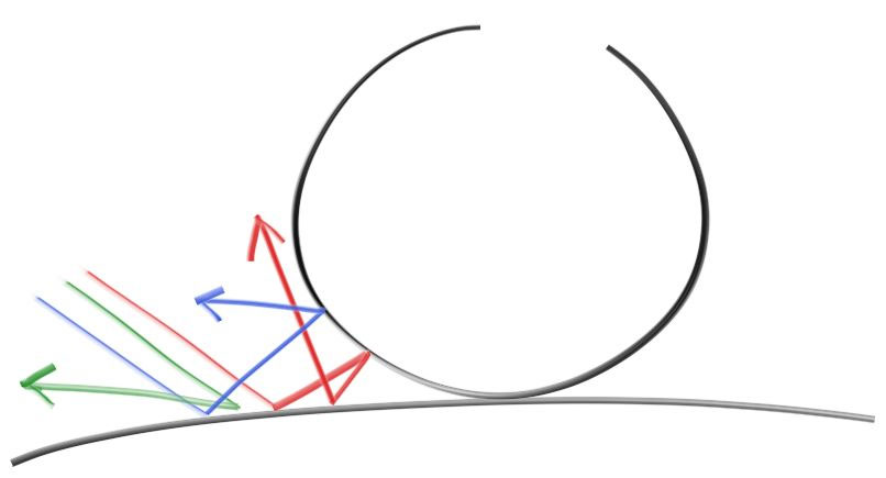
They also might be absorbed rather than reflected. The darker the surface, the more likely absorption is. (That’s why it is dark!) Really any algorithm that randomizes direction will produce surfaces that look matte. One of the simplest ways to do this turns out to be exactly correct for ideal diffuse surfaces. (I used to do it as a lazy hack that approximates mathematically ideal Lambertian.)

并且大部分的光线都会被吸收, 而不是被反射。表面越暗, 吸收就越有可能发生。我们使用任意的算法生成随机的反射方向, 就能让其看上去像一个粗糙不平的漫反射材质。这里我们采用最简单的算法就能得到一个理想的漫反射表面(其实是懒得写lambertian所以用了一个数学上近似的方法)。

(Reader Vassillen Chizhov proved that the lazy hack is indeed just a lazy hack and is inaccurate. The correct representation of ideal Lambertian isn't much more work, and is presented at the end of the chapter.)

(读者Vassillen Chizhov 提供了这个方法, 虽然并不是很精确。我们会在章节最后提准确的lambertian表达式, 而且其并不会很复杂)

There are two unit radius spheres tangent to the hit point 𝑝p of a surface. These two spheres have a center of (𝐏+𝐧) and (𝐏−𝐧), where 𝐧n is the normal of the surface. The sphere with a center at (𝐏−𝐧) is considered inside the surface, whereas the sphere with center (𝐏+𝐧) is considered outside the surface. Select the tangent unit radius sphere that is on the same side of the surface as the ray origin. Pick a random point 𝐒 inside this unit radius sphere and send a ray from the hit point 𝐏 to the random point 𝐒 (this is the vector (𝐒−𝐏)):

好, 现在有两个单位球相切于点p, 这两个球体的球心为$(p+\vec N)$和$(p-\vec N)$, $\vec N$是球体表面的法向量。球心为$(p-\vec N)$的那个球在表面的内部, 球心为$(p+ \vec N)$的球在表面的外部。选择和光线原点位于表面同一侧的那个单位球, 并从球中随机选取一点s, 向量$(s−p)$就是我们要求的反射光线的方向:

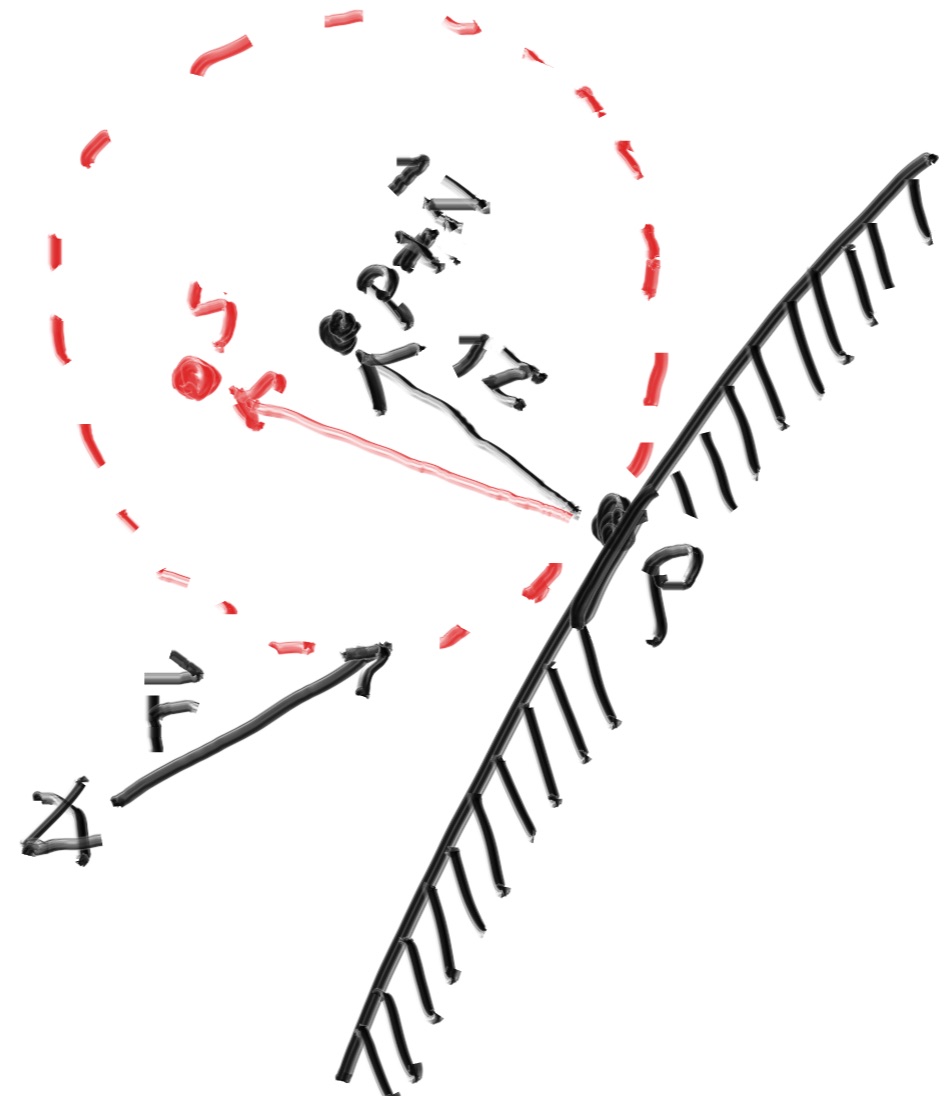
We need a way to pick a random point in a unit radius sphere. We’ll use what is usually the easiest algorithm: a rejection method. First, pick a random point in the unit cube where x, y, and z all range from −1 to +1. Reject this point and try again if the point is outside the sphere.

我们需要一个算法来生成球体内的随机点。我们会采用最简单的做法:否定法(rejection method)。首先, 在一个xyz取值范围为-1到+1的单位立方体中选取一个随机点, 如果这个点在球外就重新生成直到该点在球内。

在vec3.h中添加：

class vec3 {
  public:
    ...
    inline static vec3 random() {
        return vec3(random_double(), random_double(), random_double());
    }

    inline static vec3 random(double min, double max) {
        return vec3(random_double(min,max), random_double(min,max), random_double(min,max));
    }
}  
 
......
  
inline vec3 random_in_unit_sphere() {
    while (true) {
        auto p = vec3::random(-1,1);
        if (p.length_squared() >= 1) continue;
        return p;
    }
}  

Then update the ray_color() function to use the new random direction generator:

然后使用我们新的生成随机随机反射方向的函数来更新一下我们的ray_color()函数:

vec3 ray_color(const ray& r, const hittable& world) {
    hit_record rec;

    if (world.hit(r, 0, infinity, rec)) {
        vec3 target = rec.p + rec.normal + random_in_unit_sphere();
        return 0.5 * ray_color(ray(rec.p, target - rec.p), world);
    }

    vec3 unit_direction = unit_vector(r.direction());
    auto t = 0.5*(unit_direction.y() + 1.0);
    return (1.0-t)*vec3(1.0, 1.0, 1.0) + t*vec3(0.5, 0.7, 1.0);
}

There's one potential problem lurking here. Notice that the ray_color function is recursive. When will it stop recursing? When it fails to hit anything. In some cases, however, that may be a long time — long enough to blow the stack. To guard against that, let's limit the maximum recursion depth, returning no light contribution at the maximum depth:

这里还有个潜在的问题: 注意ray_color函数是一个递归函数。那么递归终止的条件是什么呢?当它没有击中任何东西。但是, 在某些条件下, 达到这个终止条件的时间会非常长, 长到足够爆了函数栈【译注:想象一下一条光线在一个镜子材质的密封的盒子(并不吸收光线)中反复折射, 永无尽头】。为了避免这种情况的发生, 我们使用一个变量depth限制递归层数。当递归层数达到限制值时我们终止递归, 返回黑色:【译注: 可以试试返回纯红(1,0,0), 然后渲染一下, 大致看一下是哪里在不停的发生散射】

+vec3 ray_color(const ray& r, const hittable& world, int depth) {
+    hit_record rec;

+    // If we've exceeded the ray bounce limit, no more light is gathered.
+    if (depth <= 0)
+        return vec3(0,0,0);

+    if (world.hit(r, 0, infinity, rec)) {
+        vec3 target = rec.p + rec.normal + random_in_unit_sphere();
+        return 0.5 * ray_color(ray(rec.p, target - rec.p), world, depth-1);
+   }

    vec3 unit_direction = unit_vector(r.direction());
    auto t = 0.5*(unit_direction.y() + 1.0);
    return (1.0-t)*vec3(1.0, 1.0, 1.0) + t*vec3(0.5, 0.7, 1.0);
}
...
int main() {
    const int image_width = 200;
    const int image_height = 100;
    const int samples_per_pixel = 100;
+   const int max_depth = 50;

    ...
    for (int j = image_height-1; j >= 0; --j) {
        std::cerr << "\rScanlines remaining: " << j << ' ' << std::flush;
        for (int i = 0; i < image_width; ++i) {
            vec3 color(0, 0, 0);
            for (int s = 0; s < samples_per_pixel; ++s) {
                auto u = (i + random_double()) / image_width;
                auto v = (j + random_double()) / image_height;
                ray r = cam.get_ray(u, v);
+               color += ray_color(r, world, max_depth);
            }
            color.write_color(std::cout, samples_per_pixel);
        }
    }

    std::cerr << "\nDone.\n";
}

This gives us:

我们会得到:

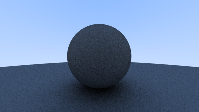
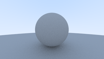
Note the shadowing under the sphere. This picture is very dark, but our spheres only absorb half the energy on each bounce, so they are 50% reflectors. If you can’t see the shadow, don’t worry, we will fix that now. These spheres should look pretty light (in real life, a light grey). The reason for this is that almost all image viewers assume that the image is “gamma corrected”, meaning the 0 to 1 values have some transform before being stored as a byte. There are many good reasons for that, but for our purposes we just need to be aware of it. To a first approximation, we can use “gamma 2” which means raising the color to the power 1/𝑔𝑎𝑚𝑚𝑎, or in our simple case ½, which is just square-root:

注意球下面是有影子的。这个图片非常的暗, 但是我们的球在散射的时候只吸收了一半的能量。如果你看不见这个阴影, 别担心, 我们现在来修复一下。现实世界中的这个球明显是应该更加亮一些的。这是因为所有的看图软件都默认图像已经经过了伽马校正(gamma corrected)。即在图片存入字节之前, 颜色值发生了一次转化。这么做有许多好处, 但这并不是我们这里所讨论的重点。我们使用”gamma 2”空间, 就意味着最终的颜色值要加上指数1/gamma, 在我们的例子里就是 ½, 即开平方根:

void write_color(std::ostream &out, int samples_per_pixel) {
    // Divide the color total by the number of samples and gamma-correct
    // for a gamma value of 2.0.
    auto scale = 1.0 / samples_per_pixel;
    auto r = sqrt(scale * e[0]);
    auto g = sqrt(scale * e[1]);
    auto b = sqrt(scale * e[2]);

    // Write the translated [0,255] value of each color component.
    out << static_cast<int>(256 * clamp(r, 0.0, 0.999)) << ' '
        << static_cast<int>(256 * clamp(g, 0.0, 0.999)) << ' '
        << static_cast<int>(256 * clamp(b, 0.0, 0.999)) << '\n';
}

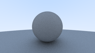
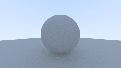
That yields light grey, as we desire:

好了, 现在看上去更灰了, 如我们所愿:

There’s also a subtle bug in there. Some of the reflected rays hit the object they are reflecting off of not at exactly 𝑡=0, but instead at 𝑡=−0.0000001 or 𝑡=0.00000001 or whatever floating point approximation the sphere intersector gives us. So we need to ignore hits very near zero:

这里还有个不太重要的潜在bug。有些物体反射的光线会在t=0时再次击中自己。然而由于精度问题, 这个值可能是t=−0.000001或者是t=0.0000000001或者任意接近0的浮点数。所以我们要忽略掉0附近的一部分范围, 防止物体发出的光线再次与自己相交。【译注: 小心自相交问题】

if (world.hit(r, 0.001, infinity, rec)) {

This gets rid of the shadow acne problem. Yes it is really called that.

这样我们就能避免阴影痤疮(shadow ance)的产生。是滴, 这种现象的确是叫这个名字。

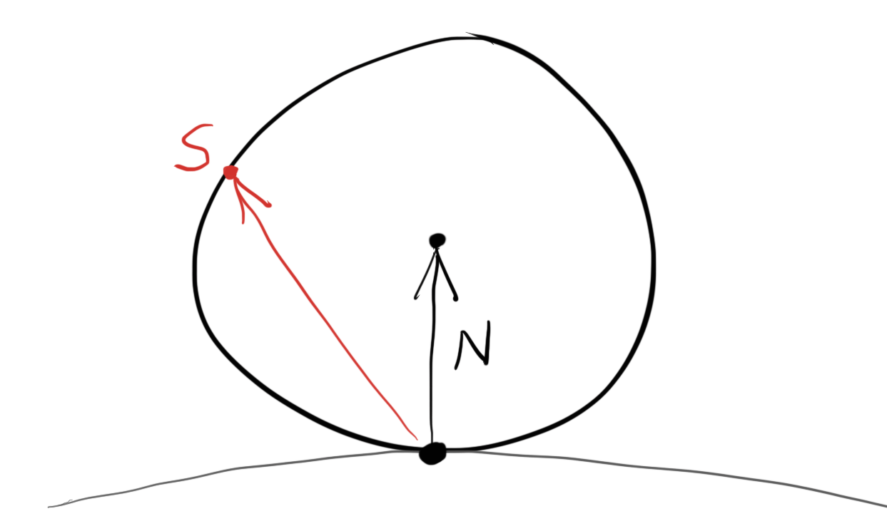
The rejection method presented here produces random points in the unit ball offset along the surface normal. This corresponds to picking directions on the hemisphere with high probability close to the normal, and a lower probability of scattering rays at grazing angles. This distribution scales by the cos3(𝜙) where 𝜙 is the angle from the normal. This is useful since light arriving at shallow angles spreads over a larger area, and thus has a lower contribution to the final color.

拒绝法生成的点是单位球体积内的的随机点, 这样生成的向量大概率上会和法线方向相近, 并且极小概率会沿着入射方向反射回去。这个分布律的表达式有一个cos3(ϕ)cos3⁡(ϕ)的系数, 其中 ϕϕ 是反射光线距离法向量的夹角。这样当光线从一个离表面很小的角度射入时, 也会散射到一片很大的区域, 对最终颜色值的影响也会更低。

However, we are interested in a Lambertian distribution, which has a distribution of cos(𝜙). True Lambertian has the probability higher for ray scattering close to the normal, but the distribution is more uniform. This is achieved by picking random points on the surface of the unit sphere, offset along the surface normal. Picking random points on the unit sphere can be achieved by picking random points in the unit sphere, and then normalizing those.

然而, 事实上的lambertian的分布律并不是这样的, 它的系数是cos(ϕ)cos⁡(ϕ)。真正的lambertian散射后的光线距离法相比较近的概率会更高, 但是分布律会更加均衡。这是因为我们选取的是单位球面上的点。我们可以通过在单位球内选取一个随机点, 然后将其单位化来获得该点。【译注: 然而下面的代码却用了极坐标的形式】

vec3 random_unit_vector() {
    auto a = random_double(0, 2*pi);
    auto z = random_double(-1, 1);
    auto r = sqrt(1 - z*z);
    return vec3(r*cos(a), r*sin(a), z);
}

This random_unit_vector() is a drop-in replacement for the existing random_in_unit_sphere() function.

我们使用新函数random_unit_vector()替换现存的random_unit_sphere():

vec3 ray_color(const ray& r, const hittable& world, int depth) {
    hit_record rec;

    // If we've exceeded the ray bounce limit, no more light is gathered.
    if (depth <= 0)
        return vec3(0,0,0);

    if (world.hit(r, 0.001, infinity, rec)) {
        vec3 target = rec.p + rec.normal + random_unit_vector();
        return 0.5 * ray_color(ray(rec.p, target - rec.p), world, depth-1);
    }

    vec3 unit_direction = unit_vector(r.direction());
    auto t = 0.5*(unit_direction.y() + 1.0);
    return (1.0-t)*vec3(1.0, 1.0, 1.0) + t*vec3(0.5, 0.7, 1.0);
}

After rendering we get a similar image:

我们会得到这样的图片, 和之前很相像:

It's hard to tell the difference between these two diffuse methods, given that our scene of two spheres is so simple, but you should be able to notice two important visual differences:

1. The shadows are less pronounced after the change
2. Both spheres are lighter in appearance after the change

Both of these changes are due to the more uniform scattering of the light rays, fewer rays are scattering toward the normal. This means that for diffuse objects, they will appear lighter because more light bounces toward the camera. For the shadows, less light bounces straight-up, so the parts of the larger sphere directly underneath the smaller sphere are brighter.

我们的场景太简单, 区分这两种方法是比较难的。但你应该能够注意到视觉上的一些差异:

1.阴影部分少了 2.大球和小球都变亮了

这些变化都是由散射光线的单位规整化引起的, 现在更少的光线会朝着发现方向散射。对于漫发射的物体来说, 他们会变得更亮。因为更多光线朝着摄像机反射。对于阴影部分来说, 更少的光线朝上反射, 所以小球下方的大球区域会变得更加明亮。

The initial hack presented in this book lasted a long time before it was proven to be an incorrect approximation of ideal Lambertian diffuse. A big reason that the error persisted for so long is that it can be difficult to:

1. Mathematically prove that the probability distribution is incorrect
2. Intuitively explain why a cos(𝜙) distribution is desirable (and what it would look like)

Not a lot of common, everyday objects are perfectly diffuse, so our visual intuition of how these objects behave under light can be poorly formed.

这本书很长一段时间都采用的是先前的版本, 直到后来有一天大家发现它其实只是理想lambertian漫发射的近似, 其并不正确。这个错误在本书中留存了那么长时间, 主要是因为:

1.概率分布的数学证明算错了 2.视觉上来说, 并不能直接看出cos(ϕ)的概率分配是我们所需要的

因为大家日常生活中的物体都是发生了完美的漫反射, 所以我们很难养成对光照下物体是如何表现的视觉直觉。

In the interest of learning, we are including an intuitive and easy to understand diffuse method. For the two methods above we had a random vector, first of random length and then of unit length, offset from the hit point by the normal. It may not be immediately obvious why the vectors should be displaced by the normal.

为了便于大家理解, 简单来说两种方法都选取了一个随机方向的向量, 不过一种是从单位球体内取的, 其长度是随机的, 另一种是从单位球面上取的, 长度固定为单位向量长度。为什么要采取单位球面并不是能很直观的一眼看出。

A more intuitive approach is to have a uniform scatter direction for all angles away from the hit point, with no dependence on the angle from the normal. Many of the first raytracing papers used this diffuse method (before adopting Lambertian diffuse).

另一种具有启发性的方法是, 直接从入射点开始选取一个随机的方向, 然后再判断是否在法向量所在的那个半球。在使用lambertian漫发射模型前, 早期的光线追踪论文中大部分使用的都是这个方法:

vec3 random_in_hemisphere(const vec3& normal) {
    vec3 in_unit_sphere = random_in_unit_sphere();
    if (dot(in_unit_sphere, normal) > 0.0) // In the same hemisphere as the normal
        return in_unit_sphere;
    else
        return -in_unit_sphere;
}

将我们的新函数套入ray_color()函数:

vec3 ray_color(const ray& r, const hittable& world, int depth) {
    hit_record rec;

    // If we've exceeded the ray bounce limit, no more light is gathered.
    if (depth <= 0)
        return vec3(0,0,0);

    if (world.hit(r, 0.001, infinity, rec)) {
        vec3 target = rec.p + random_in_hemisphere(rec.normal);
        return 0.5 * ray_color(ray(rec.p, target - rec.p), world, depth-1);
    }

    vec3 unit_direction = unit_vector(r.direction());
    auto t = 0.5*(unit_direction.y() + 1.0);
    return (1.0-t)*vec3(1.0, 1.0, 1.0) + t*vec3(0.5, 0.7, 1.0);
}

Gives us the following image:

我们会得到如下的图片:

Scenes will become more complicated over the course of the book. You are encouraged to switch between the different diffuse renderers presented here. Most scenes of interest will contain a disproportionate amount of diffuse materials. You can gain valuable insight by understanding the effect of different diffuse methods on the lighting of the scene.

我们的场景会随着本书的深入会变得越来越复杂。这里鼓励大家在之后都试一下这几种不同的漫反射渲染法。大多数场景都会有许多的漫反射材质。你可以从中培养出你对这几种方法的敏感程度。

金属材质

If we want different objects to have different materials, we have a design decision. We could have a universal material with lots of parameters and different material types just zero out some of those parameters. This is not a bad approach. Or we could have an abstract material class that encapsulates behavior. I am a fan of the latter approach. For our program the material needs to do two things:

1. Produce a scattered ray (or say it absorbed the incident ray).
2. If scattered, say how much the ray should be attenuated.

This suggests the abstract class:

如果我们想让不同的物体能拥有不同的材质, 我们又面临着一个设计上的抉择。我们可以设计一个宇宙无敌大材质, 这个材质里面有数不胜数的参数和材质类型可供选择。这样其实也不错, 但我们还可以设计并封装一个抽象的材质类。我反正喜欢后面一种, 对于我们的程序来说, 一个材质类应该封装两个功能进去:

1.生成散射后的光线(或者说它吸收了入射光线) 2.如果发生散射, 决定光线会变暗多少(attenuate)

下面来看一下这个抽象类:

class material {
    public:
        virtual bool scatter(
            const ray& r_in, const hit_record& rec, vec3& attenuation, ray& scattered
        ) const = 0;
};

The hit_record is to avoid a bunch of arguments so we can stuff whatever info we want in there. You can use arguments instead; it’s a matter of taste. Hittables and materials need to know each other so there is some circularity of the references. In C++ you just need to alert the compiler that the pointer is to a class, which the “class material” in the hittable class below does:

我们在函数中使用hit_record作为传入参数, 就可以不用传入一大堆变量了。当然如果你想传一堆变量进去的话也行。这也是个人喜好。当然物体和材质还要能够联系在一起。在C++中你只要告诉编译器, 我们在hit_record里面存了个材质的指针。

#ifndef HITTABLE_H
#define HITTABLE_H

#include "rtweekend.h"
#include "ray.h"
class material;

struct hit_record {
    vec3 p;
    vec3 normal;
    shared_ptr<material> mat_ptr;
    double t;
    bool front_face;


    inline void set_face_normal(const ray& r, const vec3& outward_normal) {
        front_face = dot(r.direction(), outward_normal) < 0;
        normal = front_face ? outward_normal :-outward_normal;
    }
};

class hittable {
    public:
        virtual bool hit(const ray& r, double t_min, double t_max, hit_record& rec) const = 0;
};

#endif

What we have set up here is that material will tell us how rays interact with the surface. hit_record is just a way to stuff a bunch of arguments into a struct so we can send them as a group. When a ray hits a surface (a particular sphere for example), the material pointer in the hit_record will be set to point at the material pointer the sphere was given when it was set up in main() when we start. When the ray_color() routine gets the hit_record it can call member functions of the material pointer to find out what ray, if any, is scattered.

To achieve this, we must have a reference to the material for our sphere class to returned within hit_record. See the highlighted lines below:

光线会如何与表面交互是由具体的材质所决定的。hit_record在设计上就是为了把一堆要传的参数给打包在了一起。当光线射入一个表面(比如一个球体), hit_record中的材质指针会被球体的材质指针所赋值, 而球体的材质指针是在main()函数中构造时传入的。当color()函数获取到hit_record时, 他可以找到这个材质的指针, 然后由材质的函数来决定光线是否发生散射, 怎么散射。

所以我们必须在球体的构造函数和变量区域中加入材质指针, 以便之后传给hit_record。见下面高亮的代码行:

class sphere: public hittable {
    public:
        sphere() {}
+       sphere(vec3 cen, double r, shared_ptr<material> m)
+           : center(cen), radius(r), mat_ptr(m) {};

        virtual bool hit(const ray& r, double tmin, double tmax, hit_record& rec) const;

    public:
        vec3 center;
        double radius;
+       shared_ptr<material> mat_ptr;
};

bool sphere::hit(const ray& r, double t_min, double t_max, hit_record& rec) const {
    vec3 oc = r.origin() - center;
    auto a = r.direction().length_squared();
    auto half_b = dot(oc, r.direction());
    auto c = oc.length_squared() - radius*radius;
    auto discriminant = half_b*half_b - a*c;

    if (discriminant > 0) {
        auto root = sqrt(discriminant);
        auto temp = (-half_b - root)/a;
        if (temp < t_max && temp > t_min) {
            rec.t = temp;
            rec.p = r.at(rec.t);
            vec3 outward_normal = (rec.p - center) / radius;
            rec.set_face_normal(r, outward_normal);
            rec.mat_ptr = mat_ptr;
            return true;
        }
        temp = (-half_b + root) / a;
        if (temp < t_max && temp > t_min) {
            rec.t = temp;
            rec.p = r.at(rec.t);
            vec3 outward_normal = (rec.p - center) / radius;                
            rec.set_face_normal(r, outward_normal);
+           rec.mat_ptr = mat_ptr;
            return true;
        }
    }
    return false;
}

For the Lambertian (diffuse) case we already have, it can either scatter always and attenuate by its reflectance 𝑅R, or it can scatter with no attenuation but absorb the fraction 1−𝑅1−R of the rays, or it could be a mixture of those strategies. For Lambertian materials we get this simple class:

对于我们之前写过的Lambertian(漫反射)材质来说, 这里有两种理解方法, 要么是光线永远发生散射, 每次散射衰减至R, 要么是光线并不衰减, 转而物体吸收(1-R)的光线。你也可以当成是这两种的结合。于是我们可以写出Lambertian的材质类:

class lambertian : public material {
    public:
        lambertian(const vec3& a) : albedo(a) {}

        virtual bool scatter(
            const ray& r_in, const hit_record& rec, vec3& attenuation, ray& scattered
        ) const {
            vec3 scatter_direction = rec.normal + random_unit_vector();
            scattered = ray(rec.p, scatter_direction);
            attenuation = albedo;
            return true;
        }

    public:
        vec3 albedo;
};

Note we could just as well only scatter with some probability 𝑝 and have attenuation be 𝑎𝑙𝑏𝑒𝑑𝑜/𝑝. Your choice.

If you read the code above carefully, you'll notice a small chance of mischief. If the random unit vector we generate is exactly opposite the normal vector, the two will sum to zero, which will result in a zero scatter direction vector. This leads to bad scenarios later on (infinities and NaNs), so we need to intercept the condition before we pass it on.

For smooth metals the ray won’t be randomly scattered. The key math is: how does a ray get reflected from a metal mirror? Vector math is our friend here:

注意我们也可以让光线根据一定的概率p发生散射【译注: 若判断没有散射, 光线直接消失】, 并使光线的衰减率(代码中的attenuation)为albedo/p。随你的喜好来。

对于光滑的金属材质来说, 光线是不会像漫反射那样随机散射的, 而是产生反射。关键是:对于一个金属状的镜子, 光线具体是怎么反射的呢?向量数学是我们的好朋友:

The reflected ray direction in red is just $v+2b$. In our design, 𝐧 is a unit vector, but 𝐯 may not be. The length of 𝐛 should be $v⋅n$. Because 𝐯 points in, we will need a minus sign, yielding:

反射方向的向量如图所示为$\vec V + 2\vec B$, 其中我们规定向量$\vec N$是单位向量, 但$\vec V$不一定是。向量B的长度应为$\vec V \cdot \vec N$, 因为向量$V$与向量$N$的方向相反, 这里我们需要再加上一个负号, 于是有:

vec3 reflect(const vec3& v, const vec3& n) {
    return v - 2*dot(v,n)*n;
}

The metal material just reflects rays using that formula:

金属材质使用上面的公式来计算反射方向:

class metal : public material {
    public:
        metal(const vec3& a) : albedo(a) {}

        virtual bool scatter(
            const ray& r_in, const hit_record& rec, vec3& attenuation, ray& scattered
        ) const {
            vec3 reflected = reflect(unit_vector(r_in.direction()), rec.normal);
            scattered = ray(rec.p, reflected);
            attenuation = albedo;
            return (dot(scattered.direction(), rec.normal) > 0);
        }

    public:
        vec3 albedo;
};

We need to modify the ray_color() function to use this:

我们还需要修改一下color函数:

vec3 ray_color(const ray& r, const hittable& world, int depth) {
    hit_record rec;

    // If we've exceeded the ray bounce limit, no more light is gathered.
    if (depth <= 0)
        return vec3(0,0,0);

    if (world.hit(r, 0.001, infinity, rec)) {
+       ray scattered;
+       vec3 attenuation;
+       if (rec.mat_ptr->scatter(r, rec, attenuation, scattered))
+           return attenuation * ray_color(scattered, world, depth-1);
+       return vec3(0,0,0);
    }

    vec3 unit_direction = unit_vector(r.direction());
    auto t = 0.5*(unit_direction.y() + 1.0);
    return (1.0-t)*vec3(1.0, 1.0, 1.0) + t*vec3(0.5, 0.7, 1.0);
}

现在我们给场景加入一些金属球:

int main() {
    const int image_width = 200;
    const int image_height = 100;
    const int samples_per_pixel = 100;
    const int max_depth = 50;

    std::cout << "P3\n" << image_width << " " << image_height << "\n255\n";

+   hittable_list world;

+   world.add(make_shared<sphere>(
+       vec3(0,0,-1), 0.5, make_shared<lambertian>(vec3(0.7, 0.3, 0.3))));
+
+   world.add(make_shared<sphere>(
+       vec3(0,-100.5,-1), 100, make_shared<lambertian>(vec3(0.8, 0.8, 0.0))));

+   world.add(make_shared<sphere>(vec3(1,0,-1), 0.5, make_shared<metal>(vec3(0.8, 0.6, 0.2))));
+   world.add(make_shared<sphere>(vec3(-1,0,-1), 0.5, make_shared<metal>(vec3(0.8, 0.8, 0.8))));

    camera cam;
    for (int j = image_height-1; j >= 0; --j) {
        std::cerr << "\rScanlines remaining: " << j << ' ' << std::flush;
        for (int i = 0; i < image_width; ++i) {
            vec3 color(0, 0, 0);
            for (int s = 0; s < samples_per_pixel; ++s) {
                auto u = (i + random_double()) / image_width;
                auto v = (j + random_double()) / image_height;
                ray r = cam.get_ray(u, v);
                color += ray_color(r, world, max_depth);
            }
            color.write_color(std::cout, samples_per_pixel);
        }
    }

    std::cerr << "\nDone.\n";
}

我们就能得到这样的图片:

We can also randomize the reflected direction by using a small sphere and choosing a new endpoint for the ray:

我们还可以给反射方向加入一点点随机性, 只要在算出反射向量后, 在其终点为球心的球内随机选取一个点作为最终的终点:

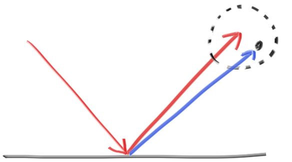
The bigger the sphere, the fuzzier the reflections will be. This suggests adding a fuzziness parameter that is just the radius of the sphere (so zero is no perturbation). The catch is that for big spheres or grazing rays, we may scatter below the surface. We can just have the surface absorb those.

当然这个球越大, 金属看上去就更加模糊(fuzzy, 或者说粗糙)。所以我们这里引入一个变量来表示模糊的程度(fuzziness)(所以当fuzz=0时不会产生模糊)。如果fuzz, 也就是随机球的半径很大, 光线可能会散射到物体内部去。这时候我们可以认为物体吸收了光线。

class metal : public material {
    public:
+       metal(const vec3& a, double f) : albedo(a), fuzz(f < 1 ? f : 1) {}

        virtual bool scatter(
            const ray& r_in, const hit_record& rec, vec3& attenuation, ray& scattered
        ) const {
            vec3 reflected = reflect(unit_vector(r_in.direction()), rec.normal);
+           scattered = ray(rec.p, reflected + fuzz*random_in_unit_sphere());
            attenuation = albedo;
            return (dot(scattered.direction(), rec.normal) > 0);//dot<0我们认为吸收
        }

    public:
        vec3 albedo;
+       double fuzz;
};

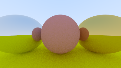
我们可以将模糊值设置为0.3和1.0, 图片会变成这样:

绝缘体材质

Clear materials such as water, glass, and diamonds are dielectrics. When a light ray hits them, it splits into a reflected ray and a refracted (transmitted) ray. We’ll handle that by randomly choosing between reflection or refraction, and only generating one scattered ray per interaction.

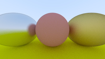
透明的材料, 例如水, 玻璃, 和钻石都是绝缘体。当光线击中这类材料时, 一条光线会分成两条, 一条发生反射, 一条发生折射。我们会采取这样的策略: 每次光线与物体相交时, 要么反射要么折射, 一次只发生一种情况,随机选取。反正最后采样次数多, 会给这些结果取个平均值。

折射部分是最难去debug的部分。我常常一开始让所有的光线只发生折射来调试。在这个项目中, 我加入了两个这样的玻璃球, 并且得到下图(我还没教你怎么弄出这样的玻璃球, 你先往下读, 一会儿你就知道了):

Is that right? Glass balls look odd in real life. But no, it isn’t right. The world should be flipped upside down and no weird black stuff. I just printed out the ray straight through the middle of the image and it was clearly wrong. That often does the job.

这图看上去是对的么? 玻璃球在现实世界中看上去和这差不多。但是, 其实这图不对。玻璃球应该会翻转上下, 也不会有这种奇怪的黑圈。我输出了图片中心的一条光线来debug, 发现它完全错了, 你调试的时候也可以这样来。

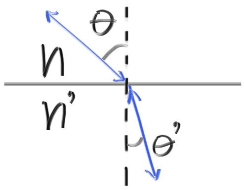
The refraction is described by Snell’s law:

$𝜂⋅sin𝜃=𝜂′⋅sin𝜃′$

Where 𝜃 and 𝜃′ are the angles from the normal, and 𝜂 and 𝜂′ (pronounced “eta” and “eta prime”) are the refractive indices (typically air = 1.0, glass = 1.3–1.7, diamond = 2.4). The geometry is:

折射法则是由Snell法则定义的：

$𝜂⋅sin𝜃=𝜂^′⋅sin𝜃^′$​

θ与θ′是入射光线与折射光线距离法相的夹角,η与η′(读作eta和eta prime)是介质的折射率(规定空气为1.0, 玻璃为1.3-1.7,钻石为2.4), 如图:

In order to determine the direction of the refracted ray, we have to solve for sin𝜃′:

$sin𝜃′= \frac{𝜂}{𝜂′}⋅sin𝜃$

为了解出折射光线的方向, 我们需要解出sinθ:

$sin𝜃′= \frac{𝜂}{𝜂′}⋅sin𝜃$

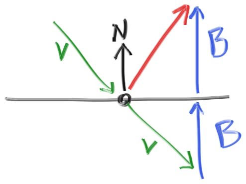
On the refracted side of the surface there is a refracted ray 𝐑′ and a normal 𝐧′, and there exists an angle, 𝜃′, between them. We can split 𝐑′ into the parts of the ray that are perpendicular to 𝐧′ and parallel to 𝐧′:

$ \mathbf{R’} = \mathbf{R’}{\bot} + \mathbf{R’}{\parallel}$​

If we solve for 𝐑′⊥ and 𝐑′∥ we get:

$ \mathbf{R’}_{\bot} = \frac{𝜂}{𝜂′}(\mathbf{R} + \cos \theta)\mathbf{n}$

$ \mathbf{R’}{\parallel} = -\sqrt{1 - |\mathbf{R’}{\bot}|^2} \mathbf{n} $

在折射介质部分有射线光线R′与法向量N′, 它们的夹角为θ′。我们可以把光线R′分解成垂直和水平与法向量N′的两个向量:

$ \mathbf{R’} = \mathbf{R’}{\bot} + \mathbf{R’}{\parallel}$

如果要解出这两个向量, 有:

$ \mathbf{R’}_{\bot} = \frac{𝜂}{𝜂′}(\mathbf{R} + \cos \theta)\mathbf{n}$

$ \mathbf{R’}{\parallel} = -\sqrt{1 - |\mathbf{R’}{\bot}|^2} \mathbf{n} $

You can go ahead and prove this for yourself if you want, but we will treat it as fact and move on. The rest of the book will not require you to understand the proof.

你可以自己推导,证明。我们这里先直接拿来当结论用了。这本书有些别的地方也是, 并不需要你完全会证明。【译注: 自己推推也没坏处】

We still need to solve for cos𝜃cos⁡θ. It is well known that the dot product of two vectors can be explained in terms of the cosine of the angle between them:

$a⋅b=|a||b|\cosθ$

If we restrict 𝐚 and 𝐛 to be unit vectors:

$a⋅b=\cos𝜃$​​

We can now rewrite 𝐑′⊥ in terms of known quantities:

$𝐑^′_⊥=\frac{𝜂}{𝜂′}(𝐑+(−𝐑⋅𝐧)𝐧)$

然后我们来解cosθ, 下面是著名的点乘的公式定义:

$a⋅b=|a||b|\cosθ$​​

如果我们将 $a$ 与 $b$ 归一化为单位向量:

$a⋅b=\cos𝜃$​​

于是我们可以这样表达垂直的那个向量:

$𝐑^′_⊥=\frac{𝜂}{𝜂′}(𝐑+(−𝐑⋅𝐧)𝐧)$

根据上述公式, 我们就能写出计算折射光线R′的函数:

vec3 refract(const vec3& uv, const vec3& n, double etai_over_etat) {
    auto cos_theta = dot(-uv, n);
    vec3 r_out_parallel = etai_over_etat * (uv + cos_theta * n);
    vec3 r_out_perp = - sqrt(fabs(1.0 - r_out_parallel.length_squared())) * n;
    return r_out_parallel + r_out_perp;
}

回到 main.cpp 中更改：

    // World
    hittable_list world;

    world.add(make_shared<sphere>(
            vec3(0,0,-1), 0.5, make_shared<lambertian>(vec3(0.7, 0.3, 0.3))));
    world.add(make_shared<sphere>(
            vec3(0,-100.5,-1), 100, make_shared<lambertian>(vec3(0.8, 0.8, 0.0))));

+   world.add(make_shared<sphere>(
+           vec3(1,0,-1), 0.5, make_shared<dielectric>(1.5)));
    
+   world.add(make_shared<sphere>(
+           vec3(-1,0,-1), 0.5, make_shared<dielectric>(1.5)));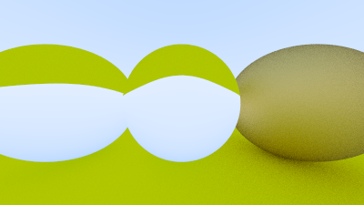

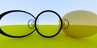
That definitely doesn't look right. One troublesome practical issue is that when the ray is in the material with the higher refractive index, there is no real solution to Snell’s law, and thus there is no refraction possible. If we refer back to Snell's law and the derivation of sin𝜃′:

$\sin𝜃^′=\frac{𝜂}{𝜂′}⋅\sin𝜃$​​

If the ray is inside glass and outside is air (𝜂=1.5 and 𝜂′=1.0):

$\sin𝜃^′=\frac{1.5}{1.0}⋅\sin𝜃$​

The value of sin𝜃′sin⁡θ′ cannot be greater than 1. So, if,

$\frac{1.5}{1.0}⋅\sin𝜃&gt;1.0$​

the equality between the two sides of the equation is broken, and a solution cannot exist. If a solution does not exist, the glass cannot refract, and therefore must reflect the ray:

现在看上去图好像不太对, 这是因为当光线从高折射律介质射入低折射率介质时, 对于上述的Snell方程可能没有实解【sinθ>1】。这时候就不会发生折射, 所以就会出现许多小黑点。我们回头看一下snell法则的式子:

$\sin𝜃^′=\frac{𝜂}{𝜂′}⋅\sin𝜃$​​

如果光线从玻璃(η=1.5)射入空气(η=1.0)

$\sin𝜃^′=\frac{1.5}{1.0}⋅\sin𝜃$​

又因为sinθ′sin⁡θ′是不可能比1大的,所以一旦这种情况发生了:

$\frac{1.5}{1.0}⋅\sin𝜃&gt;1.0$​

那就完蛋了, 方程无解了。所以我们认为光线无法发生折射的时候, 它发生了反射:

if(etai_over_etat * sin_theta > 1.0) {
    // Must Reflect
    ...
}
else {
    // Can Refract
    ...
}

Here all the light is reflected, and because in practice that is usually inside solid objects, it is called “total internal reflection”. This is why sometimes the water-air boundary acts as a perfect mirror when you are submerged.

We can solve for sin_theta using the trigonometric qualities:

$\sinθ=\sqrt{1−\cos{2θ}}$

and

$\cosθ = R ⋅ N$

这里所有的光线都不发生折射, 转而发生了反射。因为这种情况常常在实心物体的内部发生, 所以我们称这种情况被称为”全内反射”。这也当你浸入水中时, 你发现水与空气的交界处看上去像一面镜子的原因。

我们可以用三角函数解出 sin_theta：

$\sinθ=\sqrt{1−\cos{2θ}}$​

其中的 cos_theta 为：

$\cosθ = R ⋅ N$

double cos_theta = ffmin(dot(-unit_direction, rec.normal), 1.0);
double sin_theta = sqrt(1.0 - cos_theta*cos_theta);
if(etai_over_etat * sin_theta > 1.0) {
    // Must Reflect
    ...
}
else {
    // Can Refract
    ...
}

And the dielectric material that always refracts (when possible) is:

一个在可以偏折的情况下总是偏折, 其余情况发生反射的绝缘体材质为:

class dielectric : public material {
public:
    dielectric(double ri) : ref_idx(ri) {}

    virtual bool scatter (
            const ray& r_in,const hit_record& rec,vec3& attenuation,ray& scattered
    ) const {
        double etai_over_etat;
        attenuation = vec3(1.0, 1.0, 1.0);

        if (rec.front_face) {
            etai_over_etat = 1 / ref_idx;
        } else {
            etai_over_etat = ref_idx;
        }

        vec3 unit_direction = unit_vector(r_in.direction());
+       double cos_theta = ffmin(dot(-unit_direction, rec.normal), 1.0);
+       double sin_theta = sqrt(1.0 - cos_theta * cos_theta);

+       if (etai_over_etat * sin_theta > 1.0) {
+           vec3 reflected = reflect(unit_direction, rec.normal);
+           scattered = ray(rec.p, reflected);
+           return true;
+       }

        vec3 refracted = refract(unit_direction, rec.normal, etai_over_etat);
        scattered = ray(rec.p, refracted);

        return true;
    }
public:
    double ref_idx;
};

Attenuation is always 1 — the glass surface absorbs nothing. If we try that out with these parameters:

这里的光线衰减率为1——就是不衰减, 玻璃表面不吸收光的能量。如果我们使用下面的参数:

    // World
    hittable_list world;

    world.add(make_shared<sphere>(
            vec3(0,0,-1), 0.5, make_shared<lambertian>(vec3(0.1, 0.2, 0.5))));
    world.add(make_shared<sphere>(
            vec3(0,-100.5,-1), 100, make_shared<lambertian>(vec3(0.8, 0.8, 0.0))));

    world.add(make_shared<sphere>(
           vec3(1,0,-1), 0.5, make_shared<metal>(vec3(0.8, 0.6, 0.2),0.0)));

    world.add(make_shared<sphere>(
            vec3(-1,0,-1), 0.5, make_shared<dielectric>(1.5)));

We get:

我们会得到:

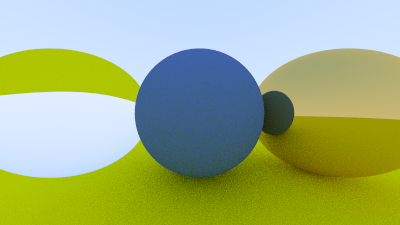
Now real glass has reflectivity that varies with angle — look at a window at a steep angle and it becomes a mirror. There is a big ugly equation for that, but almost everybody uses a cheap and surprisingly accurate polynomial approximation by Christophe Schlick. This yields our full glass material:

现实世界中的玻璃, 发生折射的概率会随着入射角而改变——从一个很狭窄的角度去看玻璃窗, 它会变成一面镜子。这个式子又丑又长, 好在我们有个数学上近似的等式, 它是由Christophe Schlick提出的:

double schlick(double cosine, double ref_idx) {
    auto r0 = (1-ref_idx) / (1+ref_idx);
    r0 = r0*r0;
    return r0 + (1-r0)*pow((1 - cosine),5);
}

这里有个简单又好用的trick, 如果你将球的半径设为负值, 形状看上去并没什么变化, 但是法相全都翻转到内部去了。所以就可以用这个特性来做出一个通透的玻璃球:【把一个小球套在大球里, 光线发生两次折射, 于是负负得正, 上下不会颠倒】:

world.add(make_shared<sphere>(vec3(0,0,-1), 0.5, make_shared<lambertian>(vec3(0.1, 0.2, 0.5))));
world.add(make_shared<sphere>(
    vec3(0,-100.5,-1), 100, make_shared<lambertian>(vec3(0.8, 0.8, 0.0))));
world.add(make_shared<sphere>(vec3(1,0,-1), 0.5, make_shared<metal>(vec3(0.8, 0.6, 0.2), 0.3)));
world.add(make_shared<sphere>(vec3(-1,0,-1), 0.5, make_shared<dielectric>(1.5)));
world.add(make_shared<sphere>(vec3(-1,0,-1), -0.45, make_shared<dielectric>(1.5)));

可自定义位置的摄像机

Cameras, like dielectrics, are a pain to debug. So I always develop mine incrementally. First, let’s allow an adjustable field of view (fov). This is the angle you see through the portal. Since our image is not square, the fov is different horizontally and vertically. I always use vertical fov. I also usually specify it in degrees and change to radians inside a constructor — a matter of personal taste.

摄像机总是和绝缘体一样难以debug。所以我总是一步步搭建我的摄像机类。首先, 我们使摄像机能调整其视野范围(field of view, fov)。fov是你的视角。因为我们的图片不是方的, 所以垂直和水平的fov值是不同的。我总是使用垂直方向的fov。并且我总是使用角度制来传参, 在构造函数中再将其转化为弧度——这也是我的个人喜好。

I first keep the rays coming from the origin and heading to the 𝑧=−1 plane. We could make it the 𝑧=−2 plane, or whatever, as long as we made ℎh a ratio to that distance. Here is our setup:

首先我让射线从原点射向z=−1平面。我们当然也可以让其射向z=−2的平面,或者其他的什么值都行, 反正h和这个距离d是成比例的。

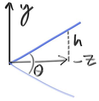
This implies $ℎ=\tan(\frac{𝜃}{2})$​. Our camera now becomes:

显然, $h=\tan(\frac{θ}{2})$。我们的摄像机类现在变成:

#ifndef RAYTRACING_DEV_CAMERA_H
#define RAYTRACING_DEV_CAMERA_H

#include "rtweekend.h"

class camera {
public:
    camera() {
        lower_left_corner = vec3(-2.0,-1.0,-1.0);
        horizontal = vec3(4.0,0.0,0.0);
        vertical = vec3(0.0,2.0,0.0);
        origin = vec3(0.0,0.0,0.0);
    }

+   camera(double vfov, double aspect) { // top to bottom, in degress
+       origin = vec3(0.0, 0.0, 0.0);

+       auto theta = degree_to_radians(vfov);
+       auto half_height = tan(theta / 2);
+       auto half_width = aspect * half_height;

+       lower_left_corner = vec3(-half_width, -half_height, -1.0);

+       horizontal = vec3(2 * half_width, 0.0, 0.0);
+       vertical = vec3(0.0, 2 * half_height, 0.0);
+   }

    ray get_ray(double u,double v) {
        return ray(origin,lower_left_corner + u * horizontal + v * vertical - origin);
    }

public:
    vec3 origin;
    vec3 lower_left_corner;
    vec3 horizontal;
    vec3 vertical;
};

#endif //RAYTRACING_DEV_CAMERA_H

When calling it with camera cam(90, aspect_ratio) and these spheres:

当我们使用一个cam(90, double(image_width)/image_height)的摄像机去拍下面的球:

    // World
    auto R = cos(pi / 4);
    hittable_list world;

    world.add(make_shared<sphere>(
            vec3(-R, 0, -1), R, make_shared<lambertian>(vec3(0, 0, 1))));
    world.add(make_shared<sphere>(
            vec3(R, 0, -1), R, make_shared<lambertian>(vec3(1, 0, 0))));

我们会得到:

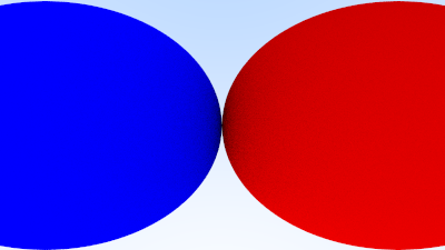
To get an arbitrary viewpoint, let’s first name the points we care about. We’ll call the position where we place the camera lookfrom, and the point we look at lookat. (Later, if you want, you could define a direction to look in instead of a point to look at.)

We also need a way to specify the roll, or sideways tilt, of the camera: the rotation around the lookat-lookfrom axis. Another way to think about it is that even if you keep lookfrom and lookat constant, you can still rotate your head around your nose. What we need is a way to specify an “up” vector for the camera. This up vector should lie in the plane orthogonal to the view direction.

为了能将我们的摄像机设置在任意位置, 我们先来给这个位置点起个名字。我们管摄像机所在的这个位置叫做 lookfrom , 我们看向的点叫做lookat(如果你不想用世界坐标下的点, 想用向量来表示这个方向的话也完全ok)。

我们还需要一个变量去描述摄像机的倾斜程度, 或者说摄像机绕着轴lookfrom - lookat旋转的角度【想象下图中红色平面绕这个轴旋转】。就好比你站直了, 但是你的头还是可以左右转动。为了去描述这个倾斜程度, 我们需要一个向量来指定摄像机坐标系的正上方方向(up vector)。这里注意:这个向量就在视线方向正交投影过来的那个平面上:

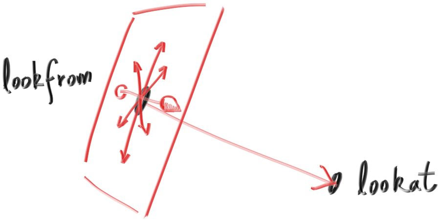
We can actually use any up vector we want, and simply project it onto this plane to get an up vector for the camera. I use the common convention of naming a “view up” (vup) vector. A couple of cross products, and we now have a complete orthonormal basis (𝑢,𝑣,𝑤) to describe our camera’s orientation.

我们可以使用任意的方向向量, 将其投影到上图的平面中来获得摄像机的up vector。我这里给他起名叫vup向量。经过一系列的点乘操作, 我们会有完整的u,v,w三个向量来描述摄像机的旋向【这里要结合着代码看与下面的图片看】。

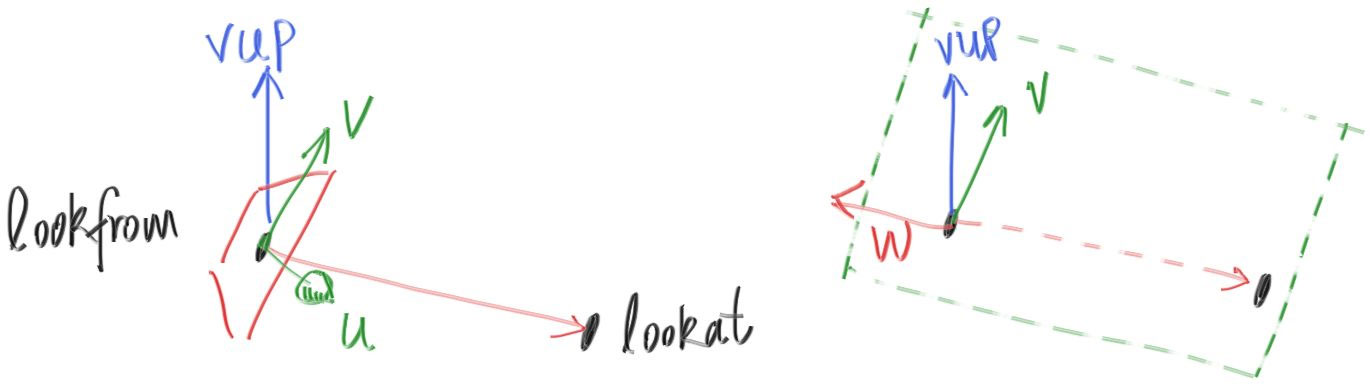
Remember that vup, v, and w are all in the same plane. Note that, like before when our fixed camera faced -Z, our arbitrary view camera faces -w. And keep in mind that we can — but we don’t have to — use world up (0,1,0) to specify vup. This is convenient and will naturally keep your camera horizontally level until you decide to experiment with crazy camera angles.

注意vup,v,w处于同一平面内。和先前我们的摄像机面对着-Z方向一样, 修改后的任意视角摄像机面对着-w方向。记得使用世界坐标系的上方向向量(0,1,0)(不是一定要用这个向量)指定vup。这样会比较方便, 并且你的摄像机镜头会保持水平。如果你想试试那些奇怪的摄像角度, 你可以放心大胆的传入别的值。

class camera {
public:
    camera() {
        lower_left_corner = vec3(-2.0,-1.0,-1.0);
        horizontal = vec3(4.0,0.0,0.0);
        vertical = vec3(0.0,2.0,0.0);
        origin = vec3(0.0,0.0,0.0);
    }

+   camera(vec3 lookfrom, vec3 lookat, vec3 vup,
            double vfov, double aspect) { // top to bottom, in degress
        origin = lookfrom;

        auto theta = degree_to_radians(vfov);
        auto half_height = tan(theta / 2);
        auto half_width = aspect * half_height;
+       vec3 w = unit_vector(lookfrom - lookat);
+       vec3 u = unit_vector(cross(vup, w));
+       vec3 v = cross(w, u);

+       lower_left_corner = origin - half_width * u - half_height * v - w;

+       horizontal = 2 * half_width * u;
+       vertical = 2 * half_height * v;
    }

    ray get_ray(double u,double v) {
        return ray(origin,lower_left_corner + u * horizontal + v * vertical - origin);
    }

public:
    vec3 origin;
    vec3 lower_left_corner;
    vec3 horizontal;
    vec3 vertical;
};

We'll change back to the prior scene, and use the new viewpoint:

现在我们就可以改变我们的视角了:

+   const auto aspect_ratio = double(image_width) / image_height;

		// World
    auto R = cos(pi / 4);
    hittable_list world;

-   world.add(make_shared<sphere>(
-           vec3(-R, 0, -1), R, make_shared<lambertian>(vec3(0, 0, 1))));
-   world.add(make_shared<sphere>(
-           vec3(R, 0, -1), R, make_shared<lambertian>(vec3(1, 0, 0))));

    world.add(make_shared<sphere>(
            vec3(0,0,-1), 0.5, make_shared<lambertian>(vec3(0.1, 0.2, 0.5))));
    world.add(make_shared<sphere>(
            vec3(0,-100.5,-1), 100, make_shared<lambertian>(vec3(0.8, 0.8, 0.0))));

    world.add(make_shared<sphere>(
           vec3(1,0,-1), 0.5, make_shared<metal>(vec3(0.8, 0.6, 0.2),0.0)));

    world.add(make_shared<sphere>(
            vec3(-1,0,-1), 0.5, make_shared<dielectric>(1.5)));

    // Camera
+   camera cam = camera(vec3(-2, 2, 1), vec3(0, 0, -1), vec3(0, 1, 0), 90, aspect_ratio);

to get:

我们会得到:

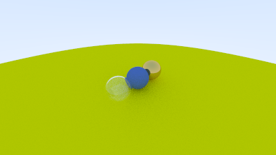
And we can change field of view:

然后我们在改变一下fov:【这里缩小了fov】

    // Camera
    camera cam = camera(vec3(-2, 2, 1), vec3(0, 0, -1), vec3(0, 1, 0), 20, aspect_ratio);

to get:

会得到:

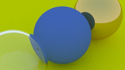
散焦模糊

Now our final feature: defocus blur. Note, all photographers will call it “depth of field” so be aware of only using “defocus blur” among friends.

终于到了我们最后的特性了: 散焦模糊(defocus blur)。基本上所有的摄影师都它叫景深(depth of field)。所以你和你朋友聊天的时候可别提什么defocus blur啊。

The reason we defocus blur in real cameras is because they need a big hole (rather than just a pinhole) to gather light. This would defocus everything, but if we stick a lens in the hole, there will be a certain distance where everything is in focus. You can think of a lens this way: all light rays coming from a specific point at the focus distance — and that hit the lens — will be bent back to a single point on the image sensor.

现实世界中的摄像机产生对焦模糊的原因是因为他们需要一个很大的孔, 而不是一个针眼大小的小孔来聚集光线。这会导致所有的东西都被散焦了。但如果我们在孔内加入一块透镜, 在一段距离内的所有物体都会被对焦。你可以这样来想象透镜:所有的光线从同一点分散射出, 击中透镜后又聚焦在图像传感器上的一个点上。

In a physical camera, the focus distance is controlled by the distance between the lens and the film/sensor. That is why you see the lens move relative to the camera when you change what is in focus (that may happen in your phone camera too, but the sensor moves). The “aperture” is a hole to control how big the lens is effectively. For a real camera, if you need more light you make the aperture bigger, and will get more defocus blur. For our virtual camera, we can have a perfect sensor and never need more light, so we only have an aperture when we want defocus blur.

在现实世界的相机中, 物体在哪里被聚焦是由透镜距离成像平面与聚焦平面这两个平面的距离所决定的。当你改变对焦设置时,相机中的这个透镜位置就会发生改变(你手机上的摄像头也是这个原理, 只不过透镜不动, 改成了成像传感器动)。快门光圈(aperture)是一个孔, 它控制这块透镜应该多大比较好。如果你需要更多的光线, 你的这个快门光圈就大一点, 景深也会随之加大。对于一个虚拟的摄像机来说, 我们只需要一个传感器就够了。所以我们只需要传入快门光圈的大小就行【即透镜大小】。

A real camera has a complicated compound lens. For our code we could simulate the order: sensor, then lens, then aperture. Then we could figure out where to send the rays, and flip the image after it's computed (the image is projected upside down on the film). Graphics people, however, usually use a thin lens approximation:

现实世界中的摄像机的透镜组是很复杂的。但对于我们写代码来说, 我们只需要模拟上述的顺序: 图像传感器, 透镜, 快门, 然后射出光线, 最后记得翻转图片(进过透镜成像会被上下翻转)。图形学中人们常常使用一块薄片透镜近似模拟:

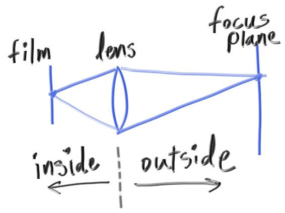
We don’t need to simulate any of the inside of the camera. For the purposes of rendering an image outside the camera, that would be unnecessary complexity. Instead, I usually start rays from the lens, and send them toward the focus plane (focus_dist away from the lens), where everything on that plane is in perfect focus.

但是我们根本不用模拟任何摄像机内部的东西, 对于我们渲染摄像机外的物体来说, 这些都没必要。我们只要从一个虚拟的透镜范围中发射光线到我们的摄像机平面就能模拟了,这个透镜与平面的距离成为焦距(focus_dist)

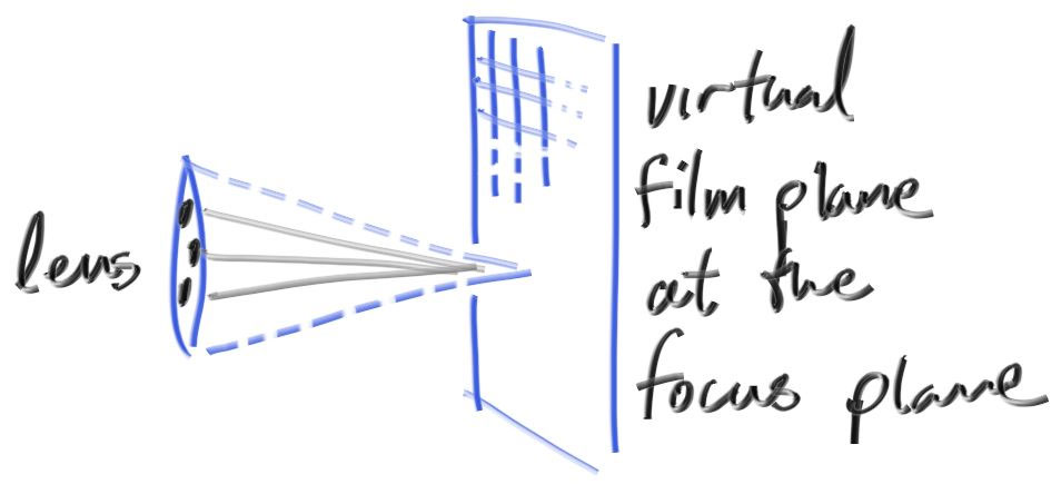
Normally, all scene rays originate from the lookfrom point. In order to accomplish defocus blur, generate random scene rays originating from inside a disk centered at the lookfrom point. The larger the radius, the greater the defocus blur. You can think of our original camera as having a defocus disk of radius zero (no blur at all), so all rays originated at the disk center (lookfrom).

之前我们所有的光线都是从lookfrom发出的, 但现在加入了散焦模糊, 所有光线都从内部的一个虚拟透镜发出, 经过lookfrom点, 这个透镜的半径越大, 图像就越模糊。你可以认为之前的摄像机, 这个半径为0。

vec3 random_in_unit_disk() {
    while (true) {
        auto p = vec3(random_double(-1,1), random_double(-1,1), 0);
        if (p.length_squared() >= 1) continue;
        return p;
    }
}

下面给出完整的 camera.h：

#ifndef RAYTRACING_DEV_CAMERA_H
#define RAYTRACING_DEV_CAMERA_H

#include "rtweekend.h"

class camera {
public:
    camera() {
        lower_left_corner = vec3(-2.0,-1.0,-1.0);
        horizontal = vec3(4.0,0.0,0.0);
        vertical = vec3(0.0,2.0,0.0);
        origin = vec3(0.0,0.0,0.0);
    }

    camera(vec3 lookfrom, vec3 lookat, vec3 vup,
+           double vfov, double aspect, double aperture, double focus_dist) { // top to bottom, in degress
        origin = lookfrom;
+       lens_radius = aperture / 2;

        auto theta = degree_to_radians(vfov);
        auto half_height = tan(theta / 2);
        auto half_width = aspect * half_height;
        w = unit_vector(lookfrom - lookat);
        u = unit_vector(cross(vup, w));
        v = cross(w, u);

-       lower_left_corner = origin - half_width * u - half_height * v - w;
+       lower_left_corner = origin
+                         - half_width * focus_dist * u
+                         - half_height * focus_dist * v
+                         - focus_dist * w;

-       horizontal = 2 * half_width * u;
-       vertical = 2 * half_height * v;
+       horizontal = 2 * half_width * focus_dist * u;
+       vertical = 2 * half_height * focus_dist * v;
    }

+   ray get_ray(double s, double t) {
+       vec3 rd = lens_radius * random_in_unit_disk();
+       vec3 offset = u * rd.x() + v * rd.y();

+       return ray(
+               origin + offset,
+               lower_left_corner + s * horizontal + t * vertical - origin - offset
+               );
+   }

public:
    vec3 origin;
    vec3 lower_left_corner;
    vec3 horizontal;
    vec3 vertical;
+   vec3 u, v, w;
+   double lens_radius;
};

#endif //RAYTRACING_DEV_CAMERA_H

Using a big aperture:

我们使用一个大大的快门光圈:

const auto aspect_ratio = double(image_width) / image_height;
...
vec3 lookfrom(3,3,2);
vec3 lookat(0,0,-1);
vec3 vup(0,1,0);
auto dist_to_focus = (lookfrom-lookat).length();
auto aperture = 2.0;

camera cam(lookfrom, lookat, vup, 20, aspect_ratio, aperture, dist_to_focus);

We get:

We get:

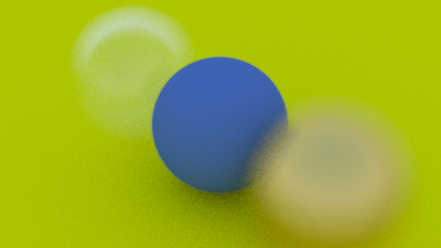
接下来学什么

首先我们在 main.cpp 把书的封面图——许多许多的随机球渲染出来:

hittable_list random_scene() {
    hittable_list world;

    world.add(make_shared<sphere>(
        vec3(0,-1000,0), 1000, make_shared<lambertian>(vec3(0.5, 0.5, 0.5))));

    int i = 1;
    for (int a = -11; a < 11; a++) {
        for (int b = -11; b < 11; b++) {
            auto choose_mat = random_double();
            vec3 center(a + 0.9*random_double(), 0.2, b + 0.9*random_double());
            if ((center - vec3(4, 0.2, 0)).length() > 0.9) {
                if (choose_mat < 0.8) {
                    // diffuse
                    auto albedo = vec3::random() * vec3::random();
                    world.add(
                        make_shared<sphere>(center, 0.2, make_shared<lambertian>(albedo)));
                } else if (choose_mat < 0.95) {
                    // metal
                    auto albedo = vec3::random(.5, 1);
                    auto fuzz = random_double(0, .5);
                    world.add(
                        make_shared<sphere>(center, 0.2, make_shared<metal>(albedo, fuzz)));
                } else {
                    // glass
                    world.add(make_shared<sphere>(center, 0.2, make_shared<dielectric>(1.5)));
                }
            }
        }
    }

    world.add(make_shared<sphere>(vec3(0, 1, 0), 1.0, make_shared<dielectric>(1.5)));

    world.add(
        make_shared<sphere>(vec3(-4, 1, 0), 1.0, make_shared<lambertian>(vec3(0.4, 0.2, 0.1))));

    world.add(
        make_shared<sphere>(vec3(4, 1, 0), 1.0, make_shared<metal>(vec3(0.7, 0.6, 0.5), 0.0)));

    return world;
}

int main() {
    ...
    auto world = random_scene();

    vec3 lookfrom(13,2,3);
    vec3 lookat(0,0,0);
    vec3 vup(0,1,0);
    auto dist_to_focus = 10.0;
    auto aperture = 0.1;

    camera cam(lookfrom, lookat, vup, 20, aspect_ratio, aperture, dist_to_focus);
    ...
}

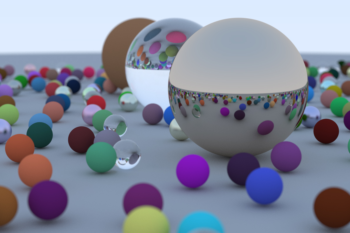
你可能会发现玻璃球没有阴影, 使得他们看上去像漂浮在空中似得。这不是bug(你在现实世界中很少有机会见到真正的玻璃球, 它们看起来的确就是这样的)。玻璃球下的那个作为地板的大球仍然能被那么多光线击中, 玻璃球下的那个作为地板的大球仍然能被那么多光线击中, 因为光线并不会被玻璃球阻挡，经由玻璃球的折射最终射向天空。【the sky is re-ordered rather than blocked. 感谢评论区Kanichiyaoba 的翻译解答】

现在你拥有一个coooool毙了的光线追踪器了! 那接下来我该何去何从呢?【标*为下本书中的内容】

1. 光照。你可以使用阴影光线来显式实现这部分, 也可以使用产生光线的材质来隐式实现*。

2. 偏移散射光线, 然后降低这些光线的权重来消除偏移。这两种都行。硬要说的话, 我偏向后者一点点。【我猜这句话是在说消除自相交所导致的阴影 即Shadow Ance, 如果有人知道这是在说什么请教教我吧！】

3. 加入三角形。大部分模型都是三角网格。模型的IO部分是最恶心的, 基本上所有人都不想自己写, 都去找别人的代码用。

4. 表面纹理*。这可以让你像贴墙纸一样把图片贴到物体上去。实现起来也很简单。

5. 固体纹理*。可以参见Ken Perlin的在线代码, Andrew Kensler的blog中也有关于这部分的信息。

6. 体积体(volumes 即雾等)*与其他介质。很Cool, 但是会改变你的代码构筑。我喜欢把体积体也设计成hittable的子类, 根据其密度来随机决定光线是否与其相交。使用这个方法, 你的渲染器甚至不用知道你渲的是体积体就渲出来了。

7. 并行优化。使用不同的随机种子, 把你的代码复制上N份跑在N个核心上,然后再求平均值。你可以分层来完成这部分工作, 比如分成N/2对, 每次平均求出N/4【为什么是N/4啊？？这翻译翻不下去了！】的图片, 然后在对这些对之间求平均值。这应该用不了多少代码【试试CUDA吧】。

记得把你渲染出的炫酷图片发给我!祝你愉快!