Self-guided Approximate Linear Programs

Last updated on: May 10, 2024

Topics: approximate dynamic programming, approximate linear programming, model-based reinforcement learning, random Fourier features, inventory management, options pricing.

Introduction

This repository hosts algorithm implementations and benchmarks discussed in the paper Self-Guided Approximate Linear Programs: Randomized Multi-Shot Approximation of Discounted Cost Markov Decision Processes authored by Parshan Pakiman, Selva Nadarajah, Negar Soheili, and Qihang Lin, available at Management Science. Specifically, this repository includes implementations of the following algorithms for computing control policies in Markov decision processes (MDPs):

Feature-based Approximate Linear Program (FALP)
Self-guided FALP
Policy-guided FALP
Least Squares Monte Carlo (Longstaff and Schwartz 2001)

Furthermore, the repository includes implementations of two algorithms for computing lower bounds on the optimal policy cost of MDPs:

Information Relaxation and Duality (Brown et al. 2010)
A heuristic based on Constraint Violation Learning (Lin et al. 2020)

Integrating lower bounds with the upper bounds derived from simulating control policies enables the computation of optimality gaps. The optimality gap of a policy is the difference between the cost of this policy and the lower bound, expressed as a percentage of the lower bound. This repository implements MDPs associated with the following applications:

Perishable inventory control
Bermudan options pricing

Note: The code in this repository is relatively general and can be extended to other MDPs to compute control policies and lower bounds.

Instruction

The following steps are tailored for macOS and Ubuntu users. Windows users may adapt and create similar instructions suitable for their operating system.

Download the repository on your local system and extract the zip file. For ease of reference, we assume the extracted files are stored in the following path: /Desktop/Self-Guided-ALPs-Discounted-Cost-master.
Open Terminal on your machine and run the following code:
```
cd  /Desktop/Self-Guided-ALPs-Discounted-Cost-master
```
Please check the version of your Python. For example, run the code below:
```
python3 --version
```
Please confirm that Python 3.10 or above is installed on your machine. There are different ways to install Python. We leave this step to the user's discretion.
Create a virtual Python environment and name it ALP. For example, use the following code:
```
python -m venv ALP   
```
Activate the ALP environment as follows:
```
source ALP/bin/activate
```
This code relies on several Python packages. We utilize pip for their installation, but users can explore alternative methods. If choosing pip, please use the following code for its update:
```
pip install --upgrade pip
```
Please install the following libraries on the ALP environment:
- numpy
- pandas
- scipy
- numba
- tqdm
- emcee
- sampyl
- importlib
- sampyl_mcmc
- nengo
- gurobipy
For instance, run the following command to install all the above libraries:
```
python -m pip install numpy pandas scipy numba tqdm emcee sampyl importlib sampyl_mcmc nengo gurobipy
```
This repository uses Gurobi for solving large-scale linear programs. Please ensure that Gurobi (gurobipy) is installed along with its corresponding license. If you are affiliated with academia, Gurobi provides a free academic license, accessible through this page. In some cases, an error might occur when running the grbgetkey code to activate your license. Refer to this troubleshooting page for assistance with resolving this issue. If the issue persists, consider installing Gurobi using conda instead of pip. You can use the following code as an example:
```
conda install -c gurobi gurobi
grbgetkey xxxxxxxx-xxxx-xxxx-xxxx-xxxxxxxxxxxx
```
Provided that the ALP environment and Gurobi are correctly installed, you can use the following code to solve test instances of perishable inventory control applications. Please run the following code:
```
./run_PIC.sh
```
The run_PIC.sh file solves the first instance of the perishable inventory control problem using the FALP algorithm with 20 random Fourier features, where FALP is formulated using a uniform state-relevance distribution (refer to the paper and code for details). You can find the specifications (e.g., cost parameters) of this instance under the path MDP/PIC/Instances/instance_1.py. To solve this instance using an alternate algorithm, you can modify the file run_PIC.sh. For instance, changing the algo_name from FALP to SG-FALP in this file and rerunning run_PIC.sh will display the output for the self-guided FALP algorithm applied to this instance. A screenshot of the output of these algorithms is attached below: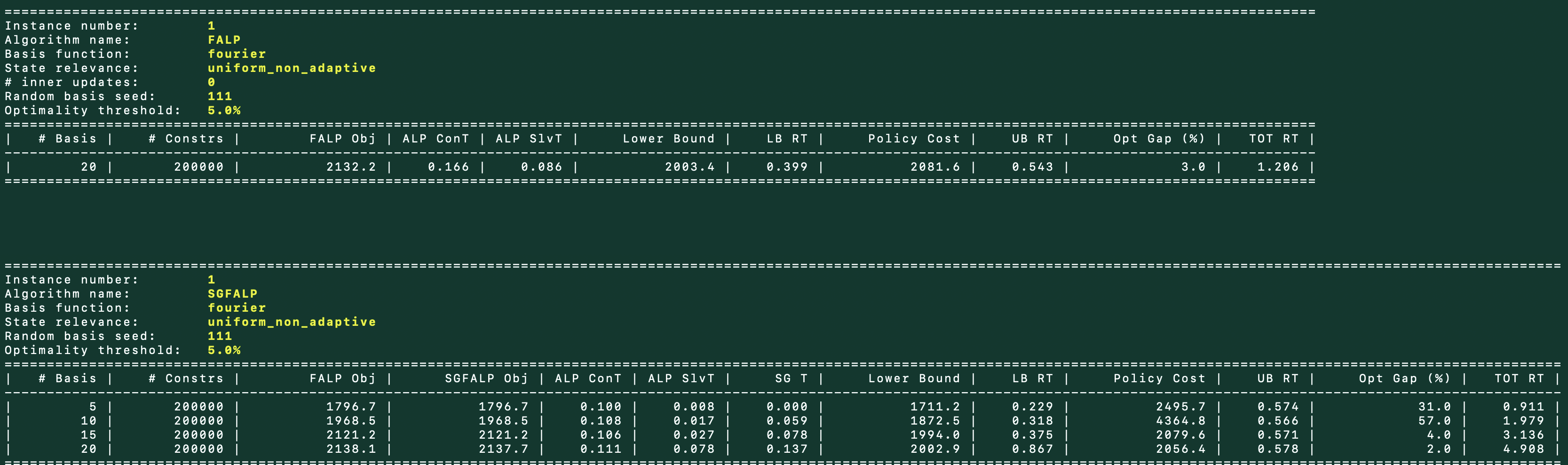
Running file run_BerOpt.sh produces the output of the algorithms for Instance 1 of the Bermudan options pricing.

Replication

The code in this repository can be directly used to replicate the tables and figures in the paper. For perishable inventory control problem instances, we consider four methods:

$\text{ALP}^{\text{LNS}}$: the standard ALP model formulated using basis functions described in Lin et al. 2020.
$\text{FALP}$: a randomized ALP model described in $\S3$ of the paper.
$\text{FALP}^{\text{PG}}$: policy-guided FALP model described in Algorithm 1 of the paper.
$\text{FALP}^{\text{SG}}$: self-guided FALP model described in Algorithm 2 of the paper.

For the Bermudan options pricing problem, we consider methods $\text{FALP}$ and $\text{FALP}^{\text{SG}}$, in addition to the following ones:

$\text{LSM}$: Least quares Monte Carlo (Longstaff and Schwartz 2001) that is implemented in file LSM.py.
$\text{ALP}^{\text{DFM}}$: the standard ALP model formulated using basis functions described in Desai et al. 2012.

We test these methods on different sets of instances described in the paper. To obtain the tables and figures in the paper, the parameters of two files, run_PIC.sh and run_BerOpt.sh, should be modified. We compute the lower and upper bounds for each instance-method pair across ten different trials. Each of these trials is specified by the value of parameter seed that is varied in {111, 222, 333, 444, 555, 666, 777, 888, 999, 1010}. For each method-instance-trial, we compute the lower and upper bounds and then the averages of these bounds across the trials for each method-instance pair. Below, we describe the other parameters in run_PIC.sh and run_BerOpt.sh to obtain each table and figur in the paper.

Table 2: Compares $\text{ALP}^{\text{LNS}}$ and $\text{FALP}$ with on 12 instances. To replicate this table, please run run_PIC.sh after modifying the following parameters:

Parameter name in `run_PIC.sh`	$\text{ALP}^{\text{LNS}}$	$\text{FALP}$
algo_name	FALP	FALP
basis_func_type	lns	fourier
max_basis_num	150	150
batch_size	150	150
state_relevance_inner_itr	0	0
instance_number	{1, 2, ..., 12}	{1, 2, ..., 12}

Please note that main.py atomatically sets the value of parameters max_basis_num and batch_size for each instance.

Table 3: Compares four models $\text{ALP}^{\text{LNS}}$, $\text{FALP}$, $\text{FALP}^{\text{PG}}$, and $\text{FALP}^{\text{SG}}$ on 6 instances. To replicate this table, please run run_PIC.sh after modifying the following parameters:

Parameter name in `run_PIC.sh`	$\text{ALP}^{\text{LNS}}$	$\text{FALP}$	$\text{FALP}^{\text{PG}}$	$\text{FALP}^{\text{SG}}$

algo_name	FALP	FALP	PG-FALP	SG-FALP
basis_func_type	lns	fourier	fourier	fourier
max_basis_num	300	300	300	300
batch_size	300	300	50	300
state_relevance_inner_itr	0	0	0	5
instance_number	{13, 14,...,18}	{13, 14,...,18}	{13, 14,...,18}	{13, 14,...,18}

Table 4: Compares four models $\text{ALP}^{\text{LNS}}$, $\text{FALP}$ with $600$ random basis functions, $\text{FALP}$ with $1000$ random basis functions, and $\text{FALP}^{\text{SG}}$ on 6 instances. To replicate this table, please run run_PIC.sh after modifying the following parameters:

Parameter name in `run_PIC.sh`	$\text{ALP}^{\text{LNS}}$	$\text{FALP}_{600}$	$\text{FALP}_{1000}$	$\text{FALP}^{\text{SG}}$

algo_name	FALP	FALP	PG-FALP	SG-FALP
basis_func_type	lns	fourier	fourier	fourier
max_basis_num	600	600	1000	600
batch_size	600	600	1000	100
state_relevance_inner_itr	0	0	0	0
instance_number	{19, 20, ..., 24}	{19, 20, ..., 24}	{19, 20, ..., 24}	{19, 20, ..., 24}

Figure 2: Depicts the violin plot of upper and lower bounds across 10 trials for 6 iterations of algorithm $\text{FALP}^{\text{SG}}$ on two instances: Instance 19 and Instance 20. Upon running this algorithm on these instances, several files will be generated under the paths Output/PIC/instance_19 and Output/PIC/instance_20. Then, one can use the plotting function in SG_FALP_progress_plot.py to obtain Figure 2 based on these files.

Table 5: Presents performance of $\text{LSM}$, $\text{ALP}^{\text{DFM}}$, $\text{FALP}$, and $\text{FALP}^{\text{SG}}$ on 9 instances. To obtain this table, please modify file run_BerOpt.sh by letting instance_number take values in {1, 2, ..., 9} and instance_number take values in {1, 2, ..., 9} and seed to take values in {111, 222, 333, 444, 555, 666, 777, 888, 999, 1010}.

Appendix

This code has undergone testing on two systems:

2021 MacBook Pro:
- CPU: M1 Pro
- Memory: 16 GB
- OS: Mac OS 14.1.2
2022 Mac Studio:
- CPU: M1 Max
- Memory: 64 GB
- OS: Mac OS 14.1.1

Below is the list of Python package versions utilized during the testing phase of this repository:

Package	Version
autograd	1.6.2
emcee	3.1.4
future	0.18.3
gurobipy	11.0.0
importlib	1.0.4
llvmlite	0.41.1
nengo	4.0.0
numba	0.58.1
numpy	1.26.2
pandas	2.1.4
pip	23.3.1
python-dateutil	2.8.2
pytz	2023.3.post1
sampyl-mcmc	0.3
scipy	1.11.4
setuptools	63.2.0
six	1.16.0
tqdm	4.66.1
tzdata	2023.3

Multi-Shot-Approximation-of-MDPs / Self-Guided-ALPs-Discounted-Cost