The libraries developed as part of this project is available on the tensorkit and bcd_tensorkit repositories. To install the relevant code, run the following lines
pip install git+https://github.com/MarieRoald/TensorKit.git@6faff50077fef2f47be9c5fdbec41bc8b16b7ec5
pip install git+https://github.com/MarieRoald/bcd_tensorkit.git@49b8fc40e3aa45b9567b11175f30d18d745a3c56
pip install condat_tv tqdm
Both the relative and absolute stopping tolerance was set to 1E-10 for all experiments.
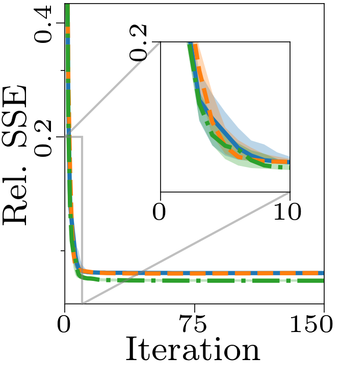
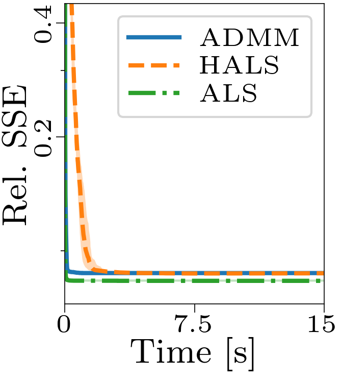
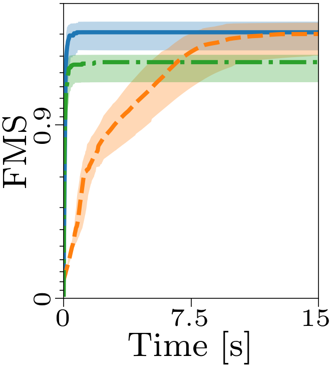
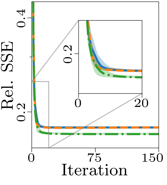
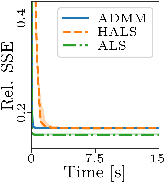
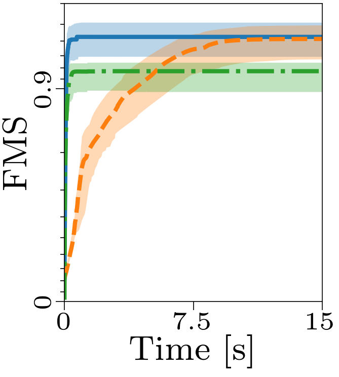
Boxplots showing the FMS and time spent until convergence with the AO-ADMM algorithm, flexible coupling with hierarchical least squares (HALS) and the traditional ALS algorithm is shown below. We have also included plots showing convergence for both noise levels.
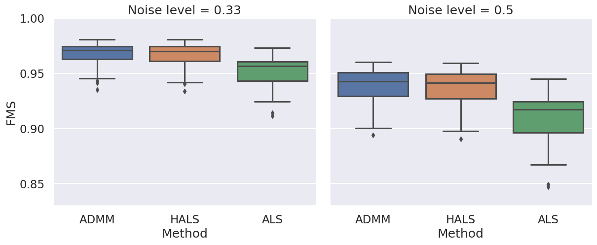 |
| FMS for the different algorithms with non-negativity constraints. |
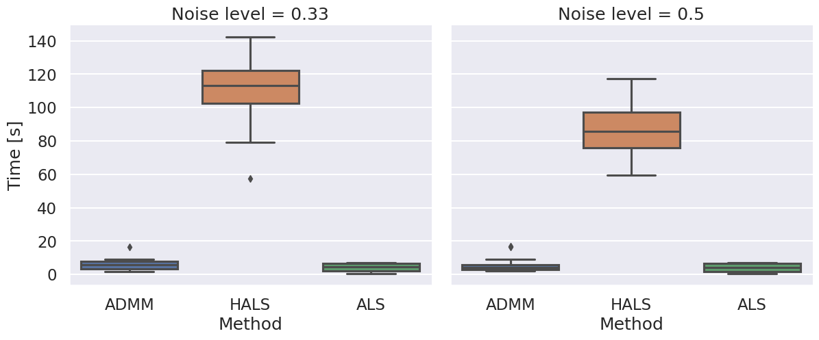 |
| Time required for convergence with the different algorithms. |
To generate the components, we fit a 3 component CP model to the Aminoacids dataset made publicly available by Rasmus Bro. We used the Emission-mode components as the blueprint for the PARAFAC2 components, shifting them cyclically to obtain the evolving factor matrices.
For the grid-search, we tested and
. The optimal regularisation parameters were
for
and
for
. We observed that for lower ridge regularisation on the non-evolving modes, the model needed higher graph Laplacian based regularisation on the evolving mode to obtain similar FMS. For both noise levels, the experiments with ridge coefficient of 1 and Laplacian regularisation strength of 1000 resulted in all-zero factor matrices. The boxplots below illustrate these results.
 |
| Results for noise level 0.33. The experiments with ridge coefficient of 1 and Laplacian regularisation strength of 100 had one outlier that obtained an FMS less than 0.6. |
 |
| Results for noise level 0.5. The experiments with ridge coefficient of 1 and Laplacian regularisation strength of 100 had one outlier that obtained an FMS less than 0.6. |
To evaluate the results, we also created animated plots of the estimated factor matrices. Below, we see the component plots from both noise levels for one of the simulated datasets.
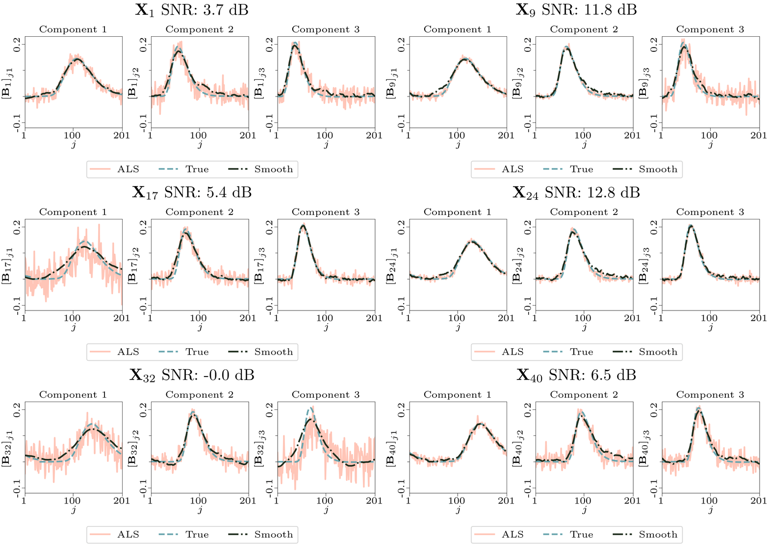 |
| Component plot for one of the datasets and noise level 0.33. |
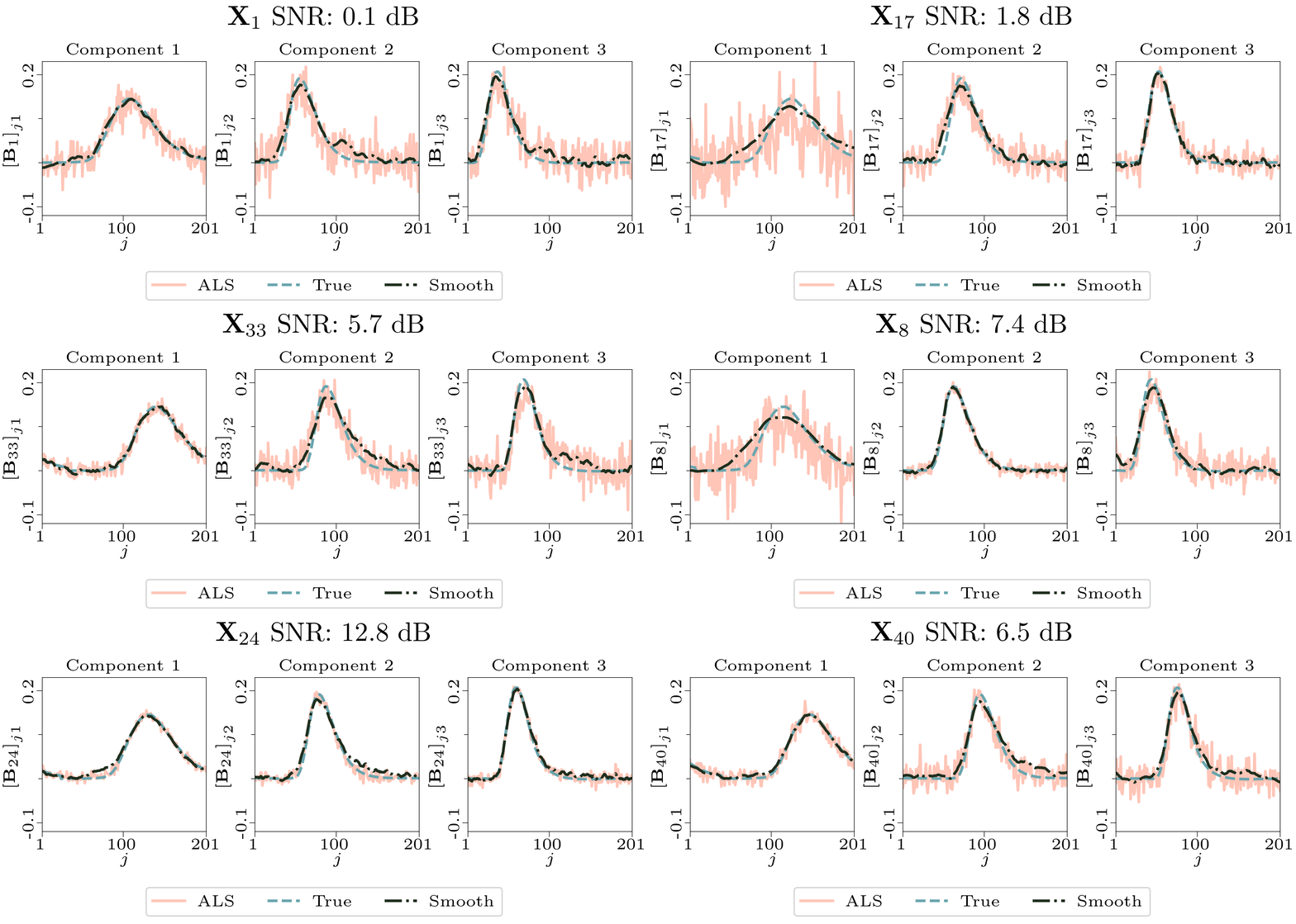 |
| Component plot for one of the datasets and noise level 0.5. |
To generate piecewise constant components with jumps that sum to zero, we used the algorithm described in the following function:
def random_piecewise_constant_vector(length, num_jumps):
    # Initialise a vector of zeros with `length/2` elements:
    derivative = np.zeros(length//2)  # // is integer divison, so 3//2 = 1, not 1.5

    # Set the first `num_jumps/2` elements of the derivative vector to a random number:
    derivative[:num_jumps//2] = np.random.standard_normal(size=num_jumps//2)

    # Concatenate the derivative vector with itself multiplied by -1 to obtain
    derivative = np.concatenate([derivative, -derivative])

    # Shuffle the derivative vector
    np.random.shuffle(derivative)  # `np.random.shuffle` modifies its input

    # Generate piecewise constant function by taking the cumulative sum of the sparse derivative vector
    piecewise_constant_function = np.cumsum(derivative)

    # Add a random offset to this function
    piecewise_constant_function += np.random.standard_normal()

    return piecewise_constant_function
For the grid search with TV regularisation, we tested and
. The optimal regularisation parameters were
for
and
for
. Again, we observed that a lower ridge regularisation strength required a higher degree of TV regularisation to obtain similar results. The boxplots below illustrate this.
 |
| Results for noise level 0.33. There were no cropped outliers for any of the parameter combinations except for those with clipped wiskers. |
We created animated plots of the estimated factor matrices. Below, we see the component plots from both noise levels for one of the simulated datasets.
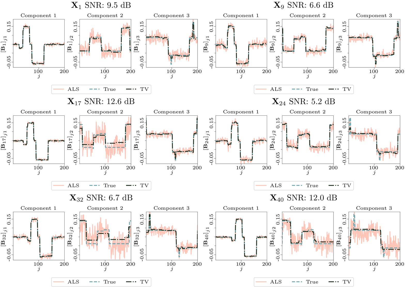 |
| Component plot for one of the datasets and noise level 0.33. |
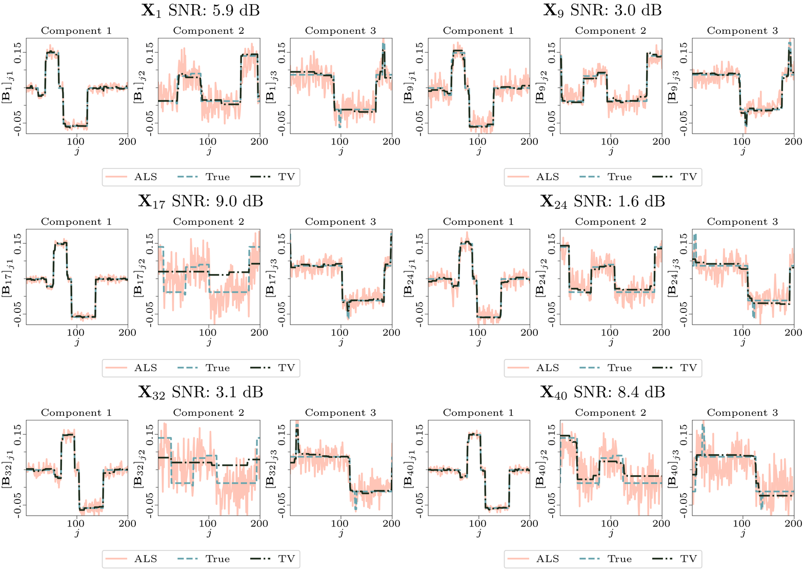 |
| Component plot for one of the datasets and noise level 0.5. |
For the results, we used the initialisation scheme listed in Table S1. Each model was initialised independently with 5 random initialisations, and the initialisation that led to the lowest regularised sum of squared errors was used for further analysis. Similar results were obtained for different initialisation schemes (e.g. using uniform initialisation for setup 2 and 3). We also obtained similar results by using the same initial parameters for both ALS and AO-ADMM for setup 2-3 and by using the same initial parameters for both ALS, AO-ADMM and HALS for setup 1.
Table S1: Initialisation scheme used for the different variables, U(0, 1) represents matrices with elements drawn from a uniform distribution between 0 and 1, and N(0, 1) represents matrices with elements drawn from a standard normal distribution. I represents an identity matrix (or the first R columns of an identity matrix).