This work is now summarised in this pre-print
Patterns and drivers of population trends on individual Breeding Bird Survey routes using spatially explicit models and route-level covariates.
Adam C. Smith, Veronica Aponte, Allison D. Binley, Amelia R. Cox, Lindsay Daly, Courtney Donkersteeg, Brandon P.M. Edwards, Willow B. English, Marie-Anne R. Hudson, David Iles, Kendall Jefferys, Barry Robinson, Christian Roy
Spatial patterns in population trends, particularly those at finer geographic scales, can help us better understand the factors driving population change in North American birds. The standard status and trend models for the North American Breeding Bird Survey (BBS) were designed to estimate trends within broad geographic strata, such as Bird Conservation Regions, U.S. states, and Canadian territories or provinces. Calculating trend estimates at the level of individual survey transects (“routes”) from the BBS allows us to explore finer spatial patterns and simultaneously estimate the effects of covariates, such as habitat-loss or annual weather, on both relative abundance and trend (changes in relative abundance through time). Here, we describe four related hierarchical Bayesian models that estimate trends for individual BBS routes, implemented in the probabilistic programing language Stan. All four models estimate route-level trends and relative abundances using a hierarchical structure that shares information among routes, and three of the models share information in a spatially explicit way. The spatial models use either an intrinsic Conditional Autoregressive structure or a distance-based Gaussian process to estimate the spatial components. We fit all four models to data for 71 species and then fit only two of the models (one spatial and one non-spatial) for an additional 216 species due to computational limitations. Leave-future-out cross-validation showed the spatial models outperformed the non-spatial model for 284 out of 287 species. For the species tested here, the best approach to modeling the spatial components depended on the species; the Gaussian Process had the highest predictive accuracy for 2/3 of the species tested here and the iCAR was better for the remaining 1/3. We also present two examples of route-level covariate analyses focused on spatial and temporal variation in habitat for Rufous Hummingbird (Selasphorus rufus) and Horned Grebe (Podiceps auritus). Covariates explain or affect patterns in the rate of population change for both species. Route-level models for BBS data are useful for visualizing spatial patterns of population change, generating hypotheses on the causes of change, comparing patterns of change among regions and species, and testing hypotheses on causes of change with relevant covariates.
A spatial model to estimate route-level trends from BBS data. One goal is to generate route-level trend estimates that could be used as data in a subsequent exploration of possible covariates of trends and abundances. These models also lend themselves well to modeling the effects of route-specific covariates (e.g., habitat change around a route) on trends and/or abundances. Finally, estimates of route-level trends provide useful site-specific information for BBS observers.
The models are written in Stan. They are based on the bbsBayes2, slope model (e.g., Sauer and Link 2011), but without the random year-effects, and with no particular stratification in which routes are nested.
We have also compared three ways of parameterizing a spatially explicit route-level trend model. We've defined two spatial models that use a neighbourhood matrix to fit an intrinsic Conditional Autoregressive (iCAR) structure: one that uses the iCAR structures only, and a second that uses a similar iCAR structure in addition to a simple random-effect to allow for greater route-specific variation in the trends (Besag York Mollie iCAR - BYM). The third spatial model is an isotropic Gaussian Process that treats the distances among the start-points for all BBS routes as a continuous spatial surface to estimate the covariance in trends and abundances.
Trends from this model represent log-linear slopes fit to the time-series of counts on a given BBS route. The model estimates the route-specific rate of change in counts for a given species, while accounting for the mean counts by the different observer(s) on the route, the start-up effect for each observers first year on a given BBS route, the mean counts at each route for an average observer, the spatial neighbourhood of each BBS route (i.e., the mean abundance for the species and the rate of change in abundance is a function of the counts on that route as well as the mean counts on routes surrounding it).
The trend at a given route may not closely match the observed counts over time, if that route has had multiple observers over the time-series, the surrounding routes have a strong and consistent pattern of change (trends), and the species data support a relatively strong influence of neighbouring regions on trend and abundance.
I've relied strongly on elements from this excellent case study in Stan:
- This intrinsic CAR model structure for the iCAR and BYM model from Mitzi Morris and co-authors.
And the Gaussian Process components were derived from case studies in Statistical Rethinking.
It's effectively a negative binomial regression model with random slopes representing the trends at each route, random intercepts representing the mean abundance (mean count) on each route, as well as the among and within observers effects (true observers, see below)
I've applied the BYM model to the BBS for ~400 species, for trends from 2004-2019. Estimated slopes, trends, and intercepts, for every route and species are available to explore in a personal Google Drive. The drive includes a readme file that explains the contents as well as trend maps for all species.
The observer effects here are random effects for each observer, not the observer-route combinations, used in the bbsBayes models. This is a new thing for the hierarchical Bayesian BBS models. The MCMC algorithm of JAGS and BUGS has a great deal of trouble separately estimating observer effects from route-level intercepts. The HMC algorithm in Stan, plus the spatially explicit estimates of the route-level intercepts, appears to have much more success.
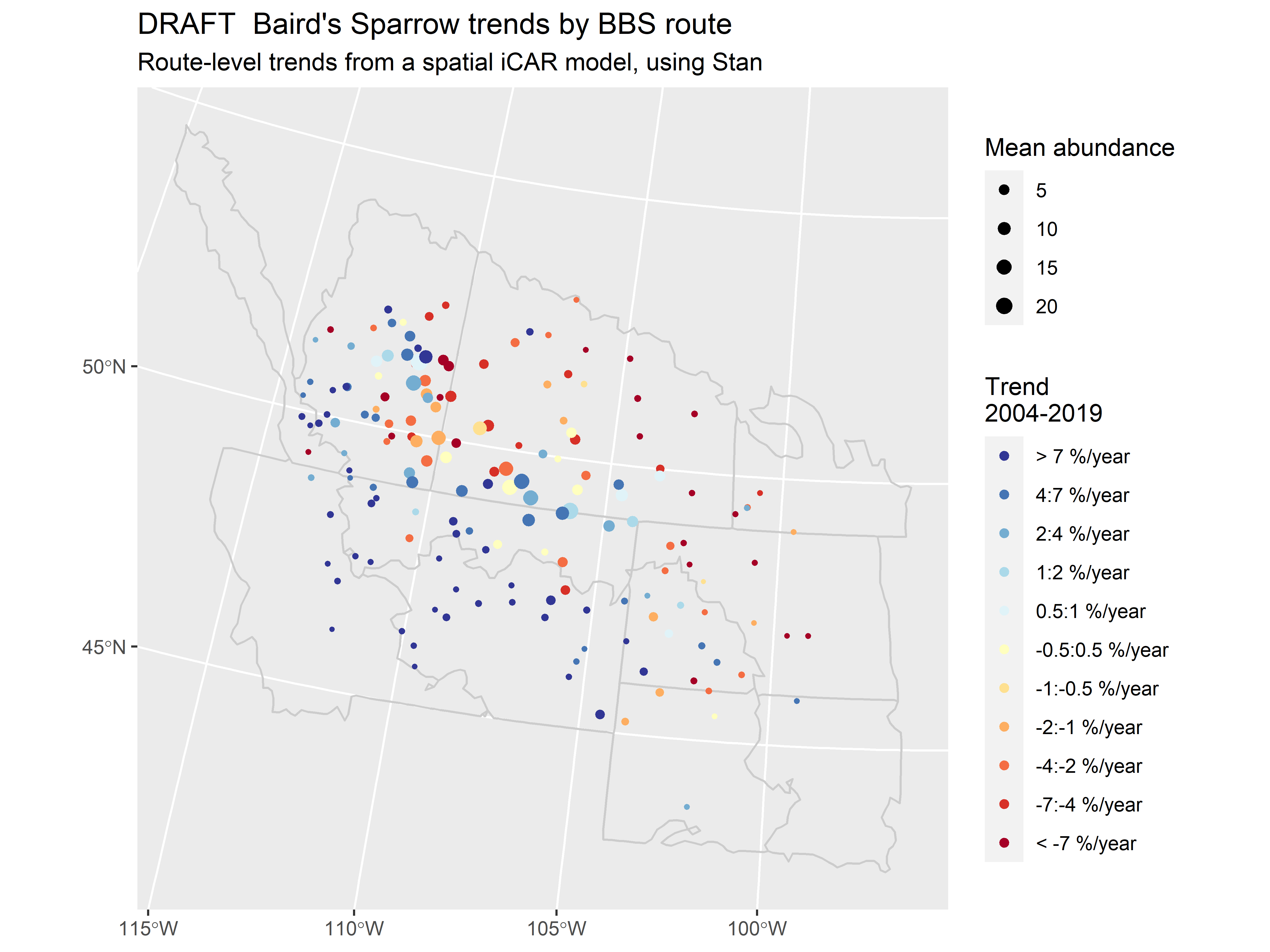
Baird's Sparrow trends in the Great Plains. Dots represent BBS routes on which Baird's Sparrow has been observed between 2004 and 2019. Over this time period, there's an interesting spatial pattern: declines in the Northeast, increases in the Southwest.
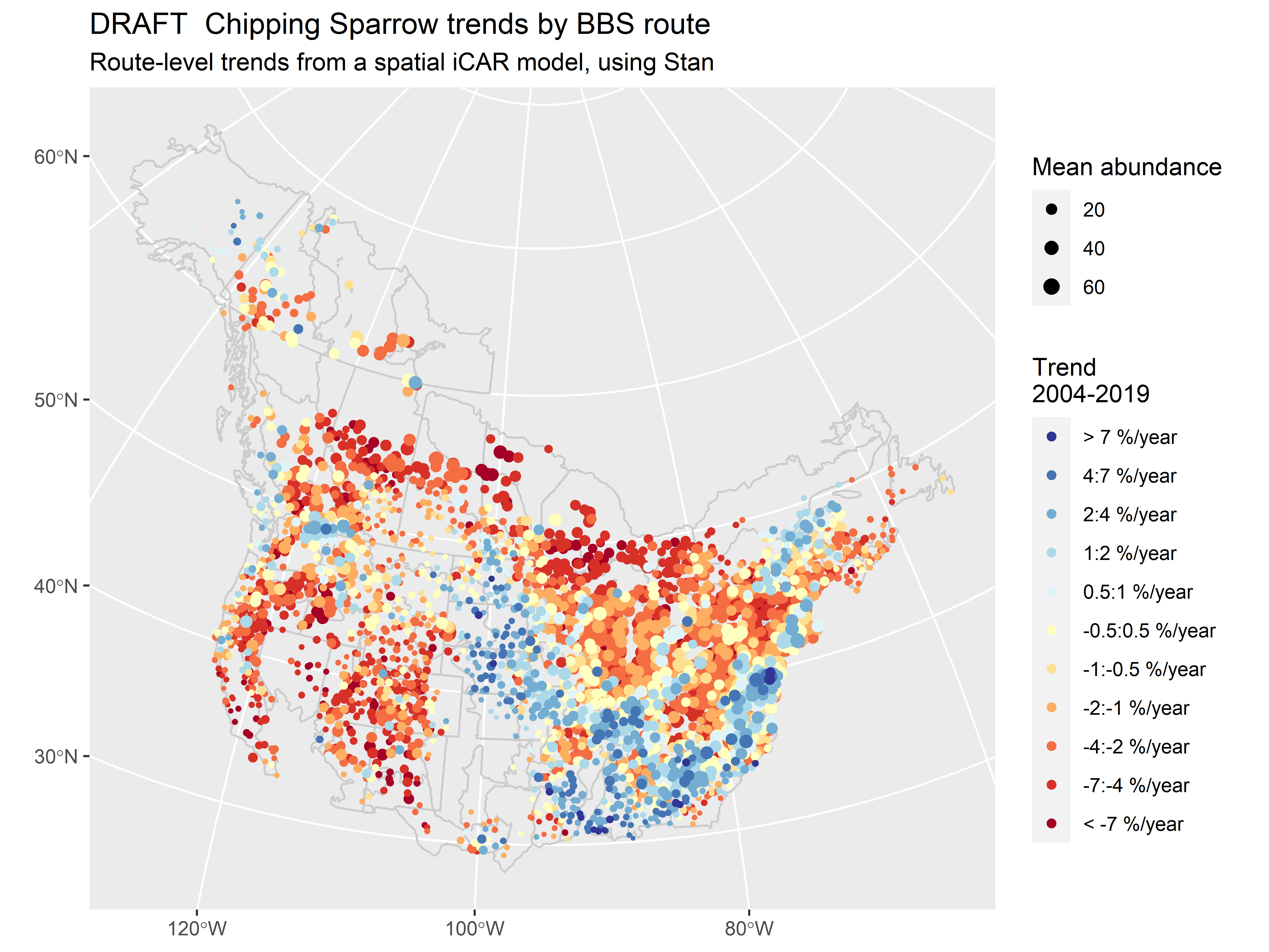
Chipping Sparrow trends over the last 15 years suggest the species has been increasing in the St-Lawrence River valley, in the southeastern portion of its range, and through some parts of the Great Plains.
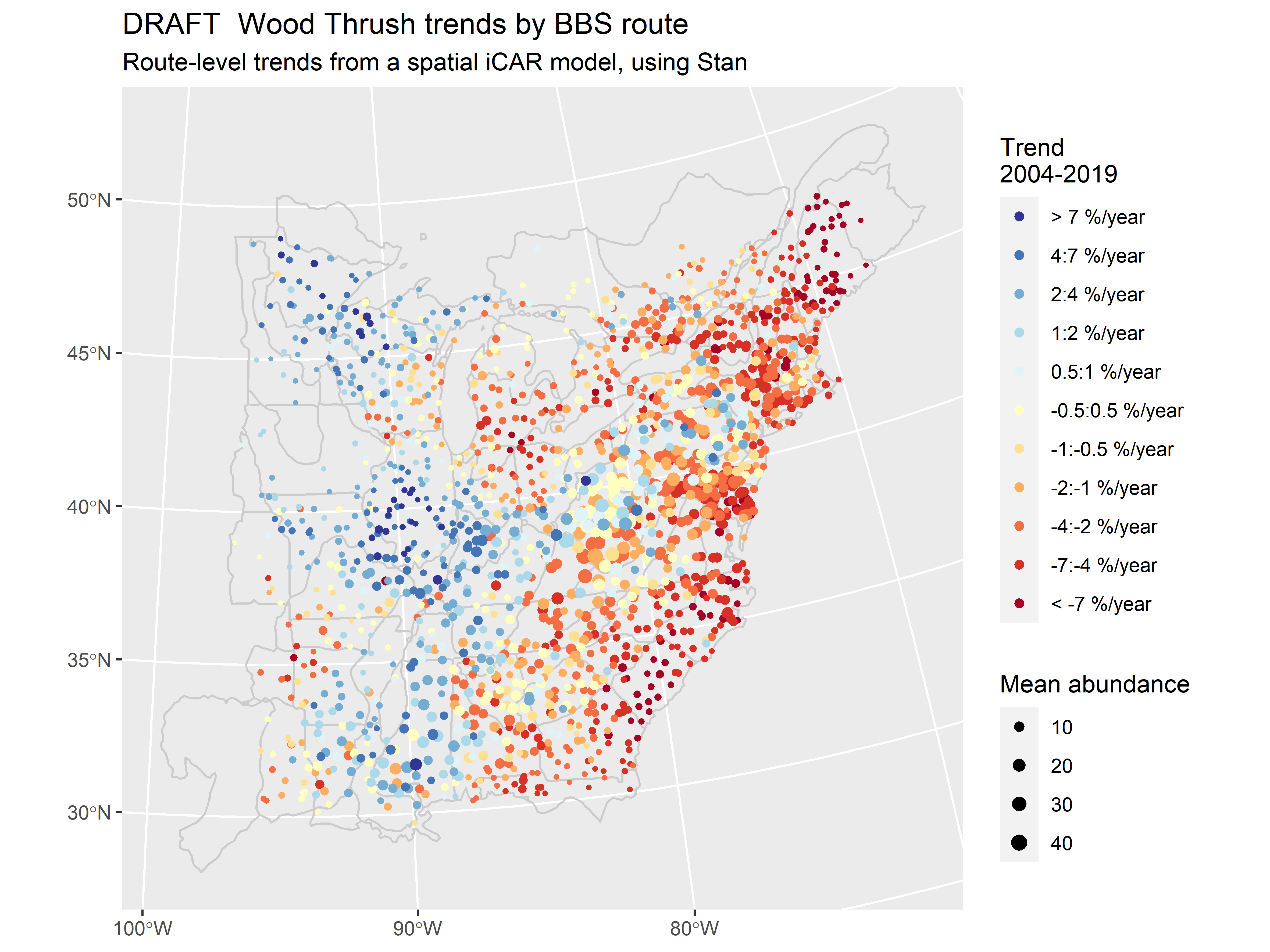
Wood Thrush trends over the last 15 years suggest the species has recently increased in the eastern parts of its range, and some portions of the Appalachians, but generally decreased in the regions where it is most abundant.


