zuzannna / BCDA

This R package is a set of tools for Bayesian analysis of categorical data, specifically 2×2 contingency tables.

Bayesian Categorical Data Analysis

This is a set of tools for Bayesian analysis of categorical data, specifically 2×2 contingency tables.

Use:

• beta_binom() for analysis using the Beta-Binomial model
  • print(), tidy(), glance(), and plot() to view the results
  • present_bbfit() if you want a nicely formatted table of summaries to include in a presentation or report
  • update() if you have additional data
• est_multinom() for estimating multinomial cell probabilities

For more information, see the Tutorial vignette.

Installing

install.packages("devtools")
devtools::install_github("bearloga/BCDA")

Usage

All examples will use the following (fake) data:

data <- matrix(c(200, 150, 250, 300), nrow = 2, byrow = TRUE)
colnames(data) <- c('Safe' ,'Dangerous')
rownames(data) <- c('Animals', 'Plants')
(data)

	Safe	Dangerous
Animals	200	150
Plants	250	300

Note that beta_binom() uses the Jeffreys prior by default.

library(BCDA) # options(digits = 2)

set.seed(0)
(fit <- beta_binom(data))

           term estimate std.error conf.low conf.high
1            p1     0.57     0.027     0.52      0.62
2            p2     0.45     0.021     0.41      0.50
3     prop_diff     0.12     0.034     0.05      0.18
4 relative_risk     1.26     0.083     1.10      1.43
5    odds_ratio     1.61     0.225     1.22      2.10

The credible intervals above are calculated using quantiles. If we have the coda package installed, we can also obtain the high posterior density intervals:

print(fit, interval_type = "HPD")

           term estimate std.error conf.low conf.high
1            p1     0.57     0.027    0.519      0.62
2            p2     0.45     0.021    0.413      0.50
3     prop_diff     0.12     0.034    0.051      0.18
4 relative_risk     1.26     0.083    1.096      1.42
5    odds_ratio     1.61     0.225    1.198      2.07

plot(fit)

Presentation of the results

The package includes a variety of functions for looking at the results from fitting a beta_binom() model. To aid in functional programming, we implemented the tidy() and glance() verbs from David Robinson's broom package for users:

library(magrittr)
fit %>% tidy %>% head(2)

  term estimate std.error conf.low conf.high
1   p1     0.57     0.027     0.52      0.62
2   p2     0.45     0.021     0.41      0.50

fit %>% glance

   n1  n2                      p1                      p2
1 350 550 57.12% (51.88%, 62.29%) 45.48% (41.38%, 49.63%)

This is perfectly okay in an interative data analysis scenario, but not when presenting the results in a report. glance() is actually a special case of the present_bbfit() function which generates all those nicely formatted credible intervals but outputs a Markdown/LaTeX-formatted table by default:

present_bbfit(fit)

Group 1	Group 2	Pr(Success) in Group 1	Pr(Success) in Group 2	Difference	Relative Risk	Odds Ratio
350	550	57.12% (51.88%, 62.29%)	45.48% (41.38%, 49.63%)	11.64% (4.96%, 18.30%)	1.26 (1.10, 1.43)	1.61 (1.22, 2.10)

The point estimates include credible intervals by default but these can be turned off:

present_bbfit(fit, conf_interval = FALSE, digits = 3)

Group 1	Group 2	Pr(Success) in Group 1	Pr(Success) in Group 2	Difference	Relative Risk	Odds Ratio
350	550	57.122%	45.479%	11.643%	1.259	1.614

Since the underlying code uses tidy() to compute the summaries, we can specify a particular credible level and the type of interval we want (e.g. highest posterior density):

present_bbfit(fit, conf_level = 0.8, interval_type = "HPD")

Group 1	Group 2	Pr(Success) in Group 1	Pr(Success) in Group 2	Difference	Relative Risk	Odds Ratio
350	550	57.12% (53.68%, 60.50%)	45.48% (42.74%, 48.10%)	11.64% (7.22%, 15.92%)	1.26 (1.15, 1.36)	1.61 (1.30, 1.87)

It also supports multiple models, which can be provided as a named or an unnamed list. See the example below.

Updating the posterior

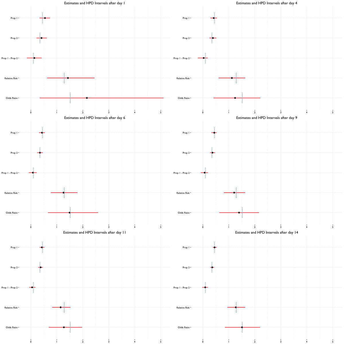
In Bayesian statistics, we can reuse a previously computed posterior as a prior if we have additional data, allowing us to update the parameter estimates as new data becomes available. Suppose we collect 40 observations from 2 groups (20 per group) on the first day of the A/B test, and 10 observations per day for the next 2 weeks. Here we see what happens when we update the posterior with additional data on a daily basis:

Example Code

fit_2 <- update(fit, x = c(100, 200), n = c(400, 600))
present_bbfit(list("Day 1" = fit, "Day 2" = fit_2))

	Group 1	Group 2	Pr(Success) in Group 1	Pr(Success) in Group 2	Difference	Relative Risk	Odds Ratio
Day 1	350	550	57.12% (51.88%, 62.29%)	45.48% (41.38%, 49.63%)	11.64% (4.96%, 18.30%)	1.26 (1.10, 1.43)	1.61 (1.22, 2.10)
Day 2	750	1150	39.96% (36.45%, 43.24%)	39.18% (36.23%, 42.01%)	0.78% (-3.73%, 5.08%)	1.02 (0.91, 1.13)	1.04 (0.85, 1.24)

If you purrrfer, you can achieve similar results the following way:

list("1" = fit, "2" = fit_2) %>%
  purrr::map_df(present_bbfit, raw = TRUE, .id = "Day") %>%
  # ...other manipulations... %>%
  knitr::kable()

Day	Group 1	Group 2	Pr(Success) in Group 1	Pr(Success) in Group 2	Difference	Relative Risk	Odds Ratio
1	350	550	57.12% (51.88%, 62.29%)	45.48% (41.38%, 49.63%)	11.64% (4.96%, 18.30%)	1.26 (1.10, 1.43)	1.61 (1.22, 2.10)
2	750	1150	39.96% (36.45%, 43.24%)	39.18% (36.23%, 42.01%)	0.78% (-3.73%, 5.08%)	1.02 (0.91, 1.13)	1.04 (0.85, 1.24)

See also

Other packages for Bayesian analysis of A/B tests include: LearnBayes (GPL), conting (GPL), bandit (GPL), testr (MIT).

---

Please note that this project is released with a Contributor Code of Conduct. By participating in this project you agree to abide by its terms.