`normflows`: A PyTorch Package for Normalizing Flows

This is a PyTorch implementation of normalizing flows. Many popular flow architectures are implemented, see the list below. The package can be easily installed via pip. The basic usage is described here, and a full documentation is available as well. There are several sample use cases implemented in the examples folder, including Glow, a VAE, and a Residual Flow.

Implemented Flows

Architecture	Reference
Planar Flow	Rezende & Mohamed, 2015
Radial Flow	Rezende & Mohamed, 2015
NICE	Dinh et al., 2014
Real NVP	Dinh et al., 2017
Glow	Kingma et al., 2018
Masked Autoregressive Flow	Papamakarios et al., 2017
Neural Spline Flow	Durkan et al., 2019
Circular Neural Spline Flow	Rezende et al., 2020
Residual Flow	Chen et al., 2019
Stochastic Normalizing Flow	Wu et al., 2020

Note that Neural Spline Flows with circular and non-circular coordinates are supported as well.

Installation

The latest version of the package can be installed via pip

pip install normflows

At least Python 3.7 is required. If you want to use a GPU, make sure that PyTorch is set up correctly by following the instructions at the PyTorch website.

To run the example notebooks clone the repository first

git clone https://github.com/VincentStimper/normalizing-flows.git

and then install the dependencies.

pip install -r requirements_examples.txt

Usage

A normalizing flow consists of a base distribution, defined in nf.distributions.base, and a list of flows, given in nf.flows. Let's assume our target is a 2D distribution. We pick a diagonal Gaussian base distribution, which is the most popular choice. Our flow shall be a Real NVP model and, therefore, we need to define a neural network for computing the parameters of the affine coupling map. One dimension is used to compute the scale and shift parameter for the other dimension. After each coupling layer we swap their roles.

import normflows as nf

# Define 2D Gaussian base distribution
base = nf.distributions.base.DiagGaussian(2)

# Define list of flows
num_layers = 32
flows = []
for i in range(num_layers):
    # Neural network with two hidden layers having 64 units each
    # Last layer is initialized by zeros making training more stable
    param_map = nf.nets.MLP([1, 64, 64, 2], init_zeros=True)
    # Add flow layer
    flows.append(nf.flows.AffineCouplingBlock(param_map))
    # Swap dimensions
    flows.append(nf.flows.Permute(2, mode='swap'))

Once they are set up, we can define a nf.NormalizingFlow model. If the target density is available, it can be added to the model to be used during training. Sample target distributions are given in nf.distributions.target.

# If the target density is not given
model = nf.NormalizingFlow(base, flows)

# If the target density is given
target = nf.distributions.target.TwoMoons()
model = nf.NormalizingFlow(base, flows, target)

The loss can be computed with the methods of the model and minimized.

# When doing maximum likelihood learning, i.e. minimizing the forward KLD
# with no target distribution given
loss = model.forward_kld(x)

# When minimizing the reverse KLD based on the given target distribution
loss = model.reverse_kld(num_samples=512)

# Optimization as usual
loss.backward()
optimizer.step()

Examples

We provide several illustrative examples of how to use the package in the examples directory. Amoung them are implementations of Glow, a VAE, and a Residual Flow. More advanced experiments can be done with the scripts listed in the repository about resampled base distributions, see its experiments folder.

Below, we consider two simple 2D examples.

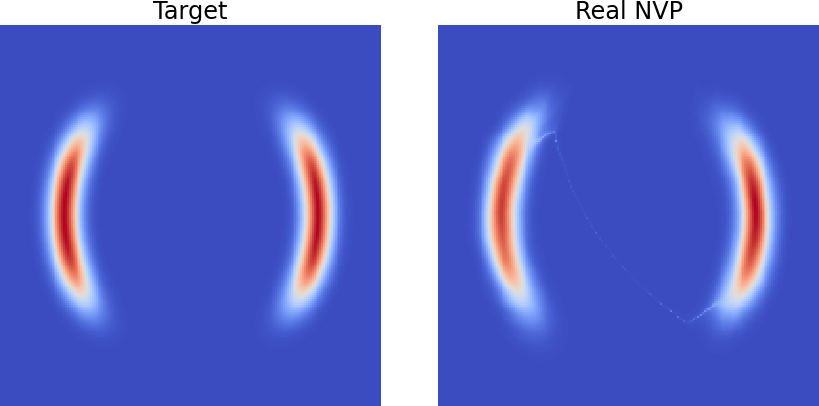
Real NVP applied to a 2D bimodal target distribution

In this notebook, which can directly be opened in Colab, we consider a 2D distribution with two half-moon-shaped modes as a target. We approximate it with a Real NVP model and obtain the following results.

Note that there might be a density filament connecting the two modes, which is due to an architectural limitation of normalizing flows, especially prominent in Real NVP. You can find out more about it in this paper.

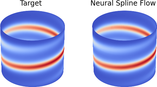
Distribution on a cylinder surface

In another example, which is available in Colab as well, we apply a Neural Spline Flow model to a distribution defined on a cylinder. The resulting density is visualized below.

This example is considered in the paper accompanying this repository.

Used by

The package has been used in several research papers, which are listed below.

Andrew Campbell, Wenlong Chen, Vincent Stimper, José Miguel Hernández-Lobato, and Yichuan Zhang. A gradient based strategy for Hamiltonian Monte Carlo hyperparameter optimization. In Proceedings of the 38th International Conference on Machine Learning, pp. 1238–1248. PMLR, 2021.

Code available on GitHub.

Vincent Stimper, Bernhard Schölkopf, José Miguel Hernández-Lobato. Resampling Base Distributions of Normalizing Flows. In Proceedings of The 25th International Conference on Artificial Intelligence and Statistics, volume 151, pp. 4915–4936, 2022.

Code available on GitHub.

Laurence I. Midgley, Vincent Stimper, Gregor N. C. Simm, Bernhard Schölkopf, José Miguel Hernández-Lobato. Flow Annealed Importance Sampling Bootstrap. arXiv preprint arXiv:2208.01893, 2022.

Code available on GitHub.

Moreover, the boltzgen package has been build upon normflows.

Citation

If you use normflows, please consider citing it as follows.

Vincent Stimper, David Liu, Andrew Campbell, Vincent Berenz, Lukas Ryll, Bernhard Schölkopf, José Miguel Hernández-Lobato: normflows: A PyTorch Package for Normalizing Flows, https://github.com/VincentStimper/normalizing-flows, 2023.

Bibtex

@software{normflows,
  author = {Vincent Stimper and David Liu and Andrew Campbell and Vincent Berenz and Lukas Ryll and Bernhard Sch{\"o}lkopf and Jos{\'e} Miguel Hern{\'a}ndez-Lobato},
  title = {normflows: {A} {P}y{T}orch {P}ackage for {N}ormalizing {F}lows},
  year = {2023},
  url = {https://github.com/VincentStimper/normalizing-flows}
}

zuhengxu / normalizing-flows