Thomas Huet, Niccolò Mazzucco, Miriam Cubas Morera, Juan Gibaja, F. Xavier Oms, António Faustino Carvalho, Ana Catarina Basilio, Elías López-Romero
NeoNet serves as a framework to investigate the transition between the Late Mesolithic and Early Neolithic periods, in the North-Central Mediterranean (loc) and European South Atlantic river basin (loc), by offering:
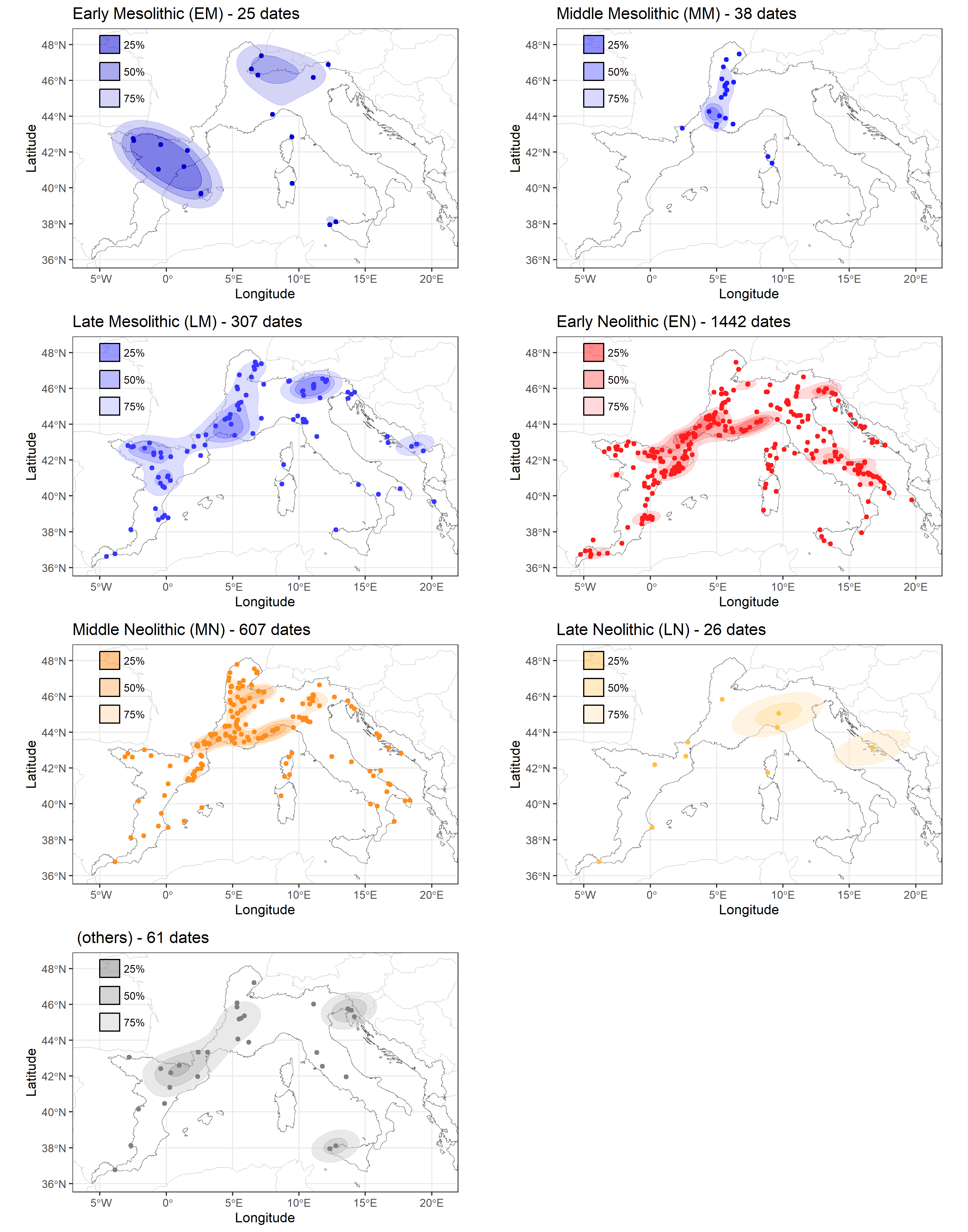
The NeoNet Med dataset filtered by periods
Studied periods are listed in the periods.tsv table:
| period | period_full_name | color |
|---|---|---|
| EM | Early Mesolithic |  |
| MM | Middle Mesolithic |  |
| LM | Late Mesolithic |  |
| LMEN | Late Mesolithic/Early Neolithic |  |
| UM | Undefined Mesolithic |  |
| EN | Early Neolithic |  |
| EMN | Early/Middle Neolithic |  |
| MN | Middle Neolithic |  |
| LN | Late Neolithic |  |
| UN | Undefined Neolithic |  |
These datasets are harvested by the c14bazAAR package, functions get_c14data("neonet") and get_c14data("neonetatl")

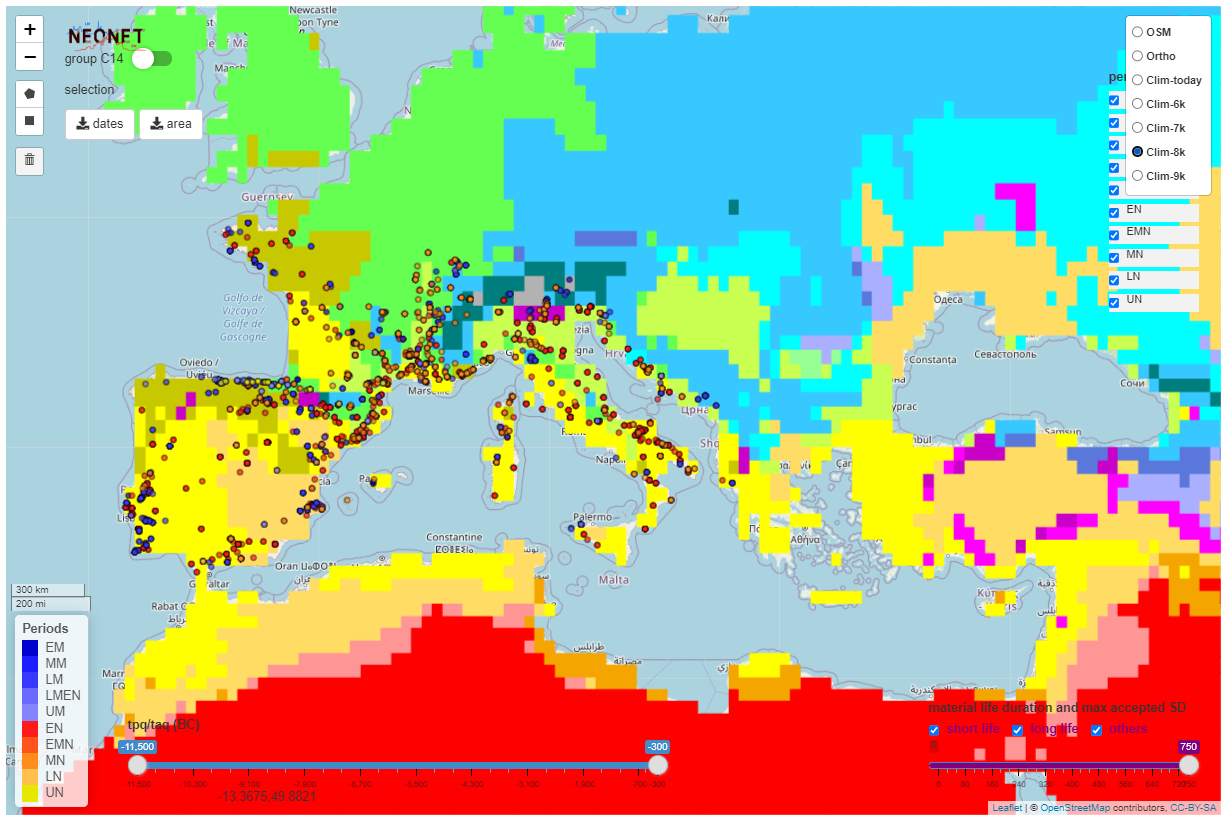
NeoNet app is an R Shiny application for mapping radiocarbon (C14). The application offers a mobile geographic window for date selection by location, various filters on chronology and date quality, a calibration window, and other tools to create a user-friendly interface supported by curated datasets of radiocarbon dates and archaeological contexts. NeoNet app is hosted on the server of the University of Pisa. This NeoNet app uses this radiocarbon dataset: https://doi.org/10.13131/archelogicadata-yb11-yb66 published as a data paper in the Journal of Open Archaeology Data and describe in this web document.
- On export action (download button), export this metadata:
- max SD
- selected periods
- dataset (Med, Atl) DOI
- timestamp
- bibliographical reference
NeoNet functions enable the handling of radiocarbon dates sourced from the dataset or exported from the interactive app. Current functions cover:
Starting by running these neo_*() functions to manage a new XLSX dataset. Sourcing functions:
source("R/neo_subset.R")
source("R/neo_bib.R")
source("R/neo_matlife.R")
source("R/neo_calib.R")
source("R/neo_merge.R")
source("R/neo_html.R")
source("R/neo_datamiss.R")
source("R/neo_datasum.R")
source("R/neo_doi.R")
Read the new dataset and bibliographic file
data.c14 <- paste0(getwd(), "/inst/extdata/", "NeoNet_atl_ELR (1).xlsx")
df.bib <- paste0(getwd(), "/inst/extdata/", "NeoNet_atl_ELR.bib")
Cleaning the dataset and making it conform to the published NeoNet dataset
df.c14 <- openxlsx::read.xlsx(data.c14)
df.c14 <- neo_subset(df.c14,
                     rm.C14Age = TRUE,
                     rm.Spatial = FALSE,
                     rm.Period = FALSE)
df.c14 <- neo_calib(df.c14)
neo_doi(df.c14)
Prepare the dataset for the Shiny application by merging it with NeoNet Med, calculating materil life duration, and HTML popup layouts
df.c14 <- neo_merge(df.c14 = df.c14,
                    data.bib = data.bib,
                    merge.bib = F)
df.c14 <- neo_matlife(df.c14)
df.c14 <- neo_html(df.c14)
Export the merged dataset
write.table(df.c14, "C:/Rprojects/neonet/R/app-dev/c14_dataset_med_x_atl.tsv",
            sep = "\t",
row.names = FALSE)Calculate basic statistics
neo_datasum(df.c14)Calculate basic statistics: missing data
neo_datamiss(df.c14)
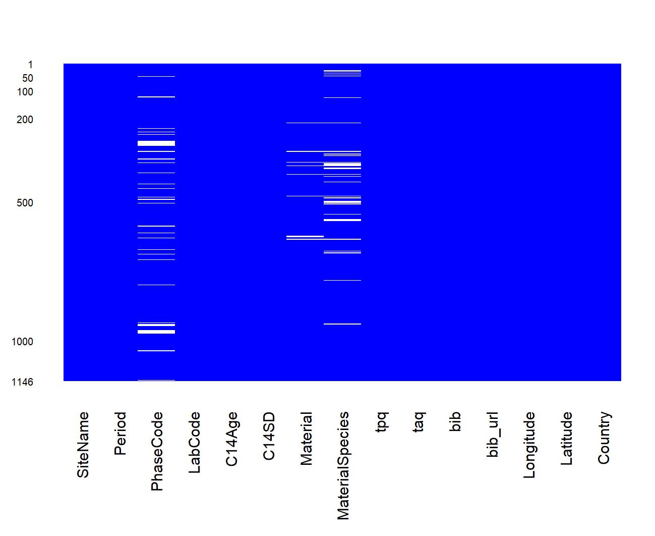
Missing data (empty cells)
Parse and align c14bazAAR data with the Neonet layout
source("R/neo_dbs_parse.R")
source("R/neo_dbs_align.R")

l.dbs <- c("calpal", "medafricarbon", "agrichange", "bda", "calpal", "radon", "katsianis")
col.c14baz <- c("sourcedb", "site", "labnr", "c14age", "c14std", "period", "culture", "lon", "lat")
df <- neo_dbs_parse(l.dbs = l.dbs,
                    col.c14baz = col.c14baz)
df.c14 <- neo_dbs_align(df)
These other databases suffer issues:
| db name | Header 2 |
|---|---|
| 14sea | No lat / lon information, spatialisation should be done on site name |
| neonet | Timeout, the server URL returns a ERR_CONNECTION_TIMED_OUT |
| p3k14c | Cultural information (culture and period) is largely missing |
Foreign dates aggregated though the c14bazAAR can be audited, for example: "Alg-40"
To retrieve dates coming from other databases (with the c14bazAAR R package) and mapped to be compliant with the Neonet format and functions, using neo_dbs_parse(), a mapping table (XLSX) created with neo_dbs_create_ref(), and neo_dbs_align():
when <- c(-9000, -4000)
where <- sf::st_read("https://raw.githubusercontent.com/zoometh/neonet/main/doc/talks/2024-simep/roi.geojson",
                     quiet = TRUE)

# collect the dates form different DBs, standardize the cultural period layout, filter on 'when' and 'where'
df <- neo_dbs_parse(l.dbs = c("bda", "medafricarbon"),
                    col.c14baz = c("sourcedb", "site", "labnr", "c14age", "c14std", "period", "culture", "lon", "lat"),
                    chr.interval.uncalBC = when,
                    roi = where)

# create the mapping file
neo_dbs_create_ref(df.all.res = df,
                   root.path = "C:/Rprojects/neonet/results",
                   outFile = "df_ref_per.xlsx")
This mapping file ref_table_per.xlsx is a reference table to map cultural assessment coming from external DBs, collected throug c14bazAAR, to the Neonet one (..., LM, EN, ...) format. This XLSX file has to be updated manually by specialists.
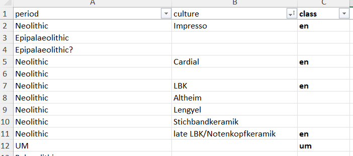
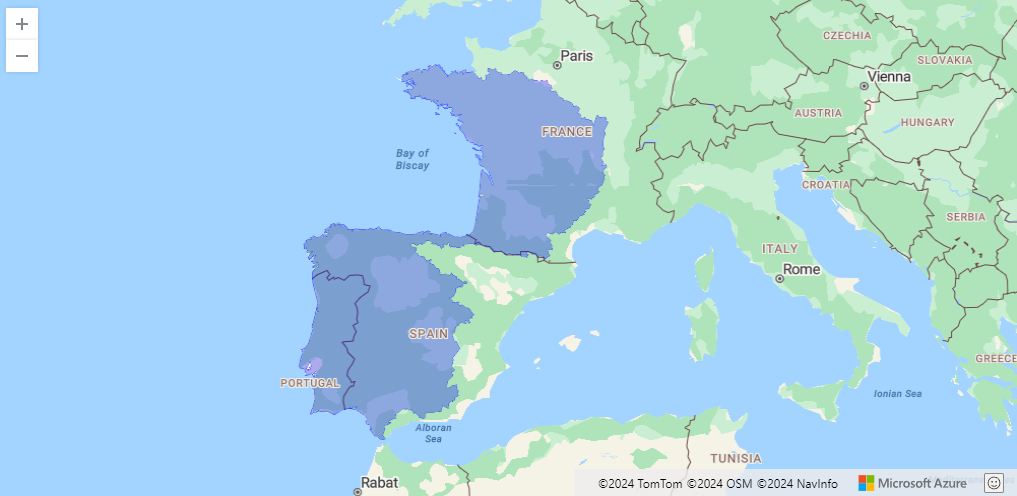
The neonet dataset over the KCC 7k
The neo_dbs_align() function reuses this mapping table.
df.c14 <- neo_dbs_align(df,
                        mapping.file = "C:/Rprojects/neonet/doc/ref_table_per.xlsx")
head(df.c14)
Gives a dataframe where all fields have been renamed to be parsed with the Neonet functions. Among this mapping the column 'Period' with, for example, MM Middle Mesolithic) maps the bda period = Mésolithique 1 and culture = Capsien ancien or Capsien typique:
| sourcedb | SiteName | LabCode | C14Age | C14SD | db_period | db_culture | Period | lon | lat |
|---|---|---|---|---|---|---|---|---|---|
| bda | Mechta el Arbi | Poz-92231 | 6600 | 80 | Mésolithique 1 | Capsien ancien | MM | 6.130900 | 36.09940 |
| bda | Mechta el Arbi | Poz-92232 | 6250 | 130 | Mésolithique 1 | Capsien ancien | MM | 6.130900 | 36.09940 |
| bda | Mechta el Arbi | Poz-92230 | 3500 | 120 | Mésolithique 1 | Capsien ancien | MM | 6.130900 | 36.09940 |
| bda | Kef Zoura D | UOC-2925 | 7787 | 48 | Mésolithique 1 | Capsien typique | MM | 7.682121 | 35.04205 |
| bda | Bortal Fakher | L-240A | 6930 | 200 | Mésolithique 1 | Capsien typique | MM | 8.176087 | 34.35480 |
| bda | Relilaï (B) | Gif-1714 | 7760 | 180 | Mésolithique 1 | Capsien typique | MM | 7.694694 | 35.04480 |
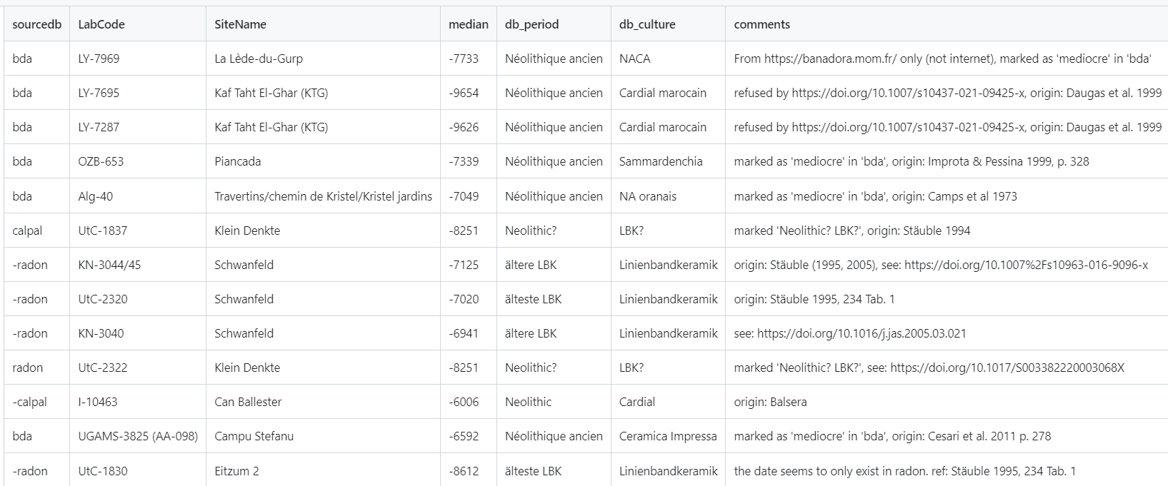
To filter aberrant dates, a combination of different function allow to retrieve the current information (once mapped to the Neonet layout) of these potential outliers and their original information (from their source database)
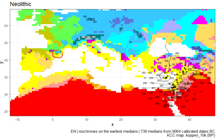
KCC and isochrone for 8000 calBC (10ka BP). Here the dates 147 (circled in red), 198 and 367 seem aberrant
source("R/neo_find_date.R")

abber.date <- neo_find_date(df = isochr$data, idf.dates = 147)
Gives:
idf sourcedb labcode     site   median period
147   calpal UBAR-31 Cova 120 -8040.05     EN
Where 147 is the contextual identifier of the date. This date comes from the calpal DB. The calibrated radiocarbon date median (-8040.05) is really too high for an EN period (Early Neolithic). Running the followin functions helps to contextualize the date.
source("R/neo_dbs_info_date_src.R")

abber.date <- neo_dbs_info_date(abber.date$labcode)
Gives:
     sourcedb LabCode SiteName   median db_period db_culture
3451   calpal UBAR-31 Cova 120 -8040.05 Neolithic Epicardial
The date 147 (aka UBAR-31) is tagged Neolithic and Epicardial in calpal. To have its full record, as it is created using the c14bazAAR package, run:
source("R/neo_dbs_info_date.R")

neo_dbs_info_date_src(db = abber.dates$sourcedb,
                      LabCode = abber.dates$LabCode)
Gives:
  sourcedb sourcedb_version method   labnr c14age c14std c13val     site sitetype    period    culture material species country
2   calpal       2020-08-20    14C UBAR-31   8550    150      0 Cova 120     <NA> Neolithic Epicardial charcoal    <NA>   Spain
    lat  lon          shortref
2 42.47 2.61 van Willigen 2006
The list of aberrant dates, for example c14_aberrant_dates.tsv, is used to discard some dates with the neo_dbs_rm_date() function
source("R/neo_dbs_rm_date.R")

df_filtered <- neo_dbs_rm_date(df.c14)
By default, dates having a dash prefix in their sourcedb column will be skipped (ex: -radon)
Screenshot of the 'c14_to_remove2.tsv' table
Plot the summed probabilty densities (SPD) of the two datasets, once df.c14 calculated. The function neo_spd() calls neo_spdplot(). The latter has been adapted from rcarbon::plot.stackCalSPD.R, to fetch NeoNet default period colors.
library(rcarbon)

source("R/neo_spd.R")
source("R/neo_spdplot.R")

neo_spd(df.c14 = df.c14)
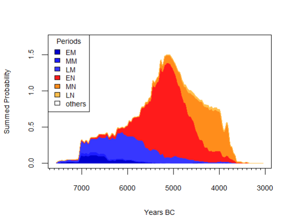
NeoNet dataset SPD with default period colors
neo_spd() can be run on a GeoJSON file exported from the NeoNet app (see "export dates" in the web document. For example neonet-data-2023-09-24.geojson, see also: isochrones
neo_spd(df.c14 = "https://raw.githubusercontent.com/zoometh/neonet/main/results/neonet-data-2023-09-24.geojson",
export = T)Create a map with isochrone contours to model the spread of Neolithic.
The file neonet-data-2023-09-24.geojson is an export from the NeoNet app (see "export dates" in the web document). This GeoJSON file can be curated in a GIS (ex: removing aberrant dates) before running the following functions (neo_isochr, neo_spd, etc.).
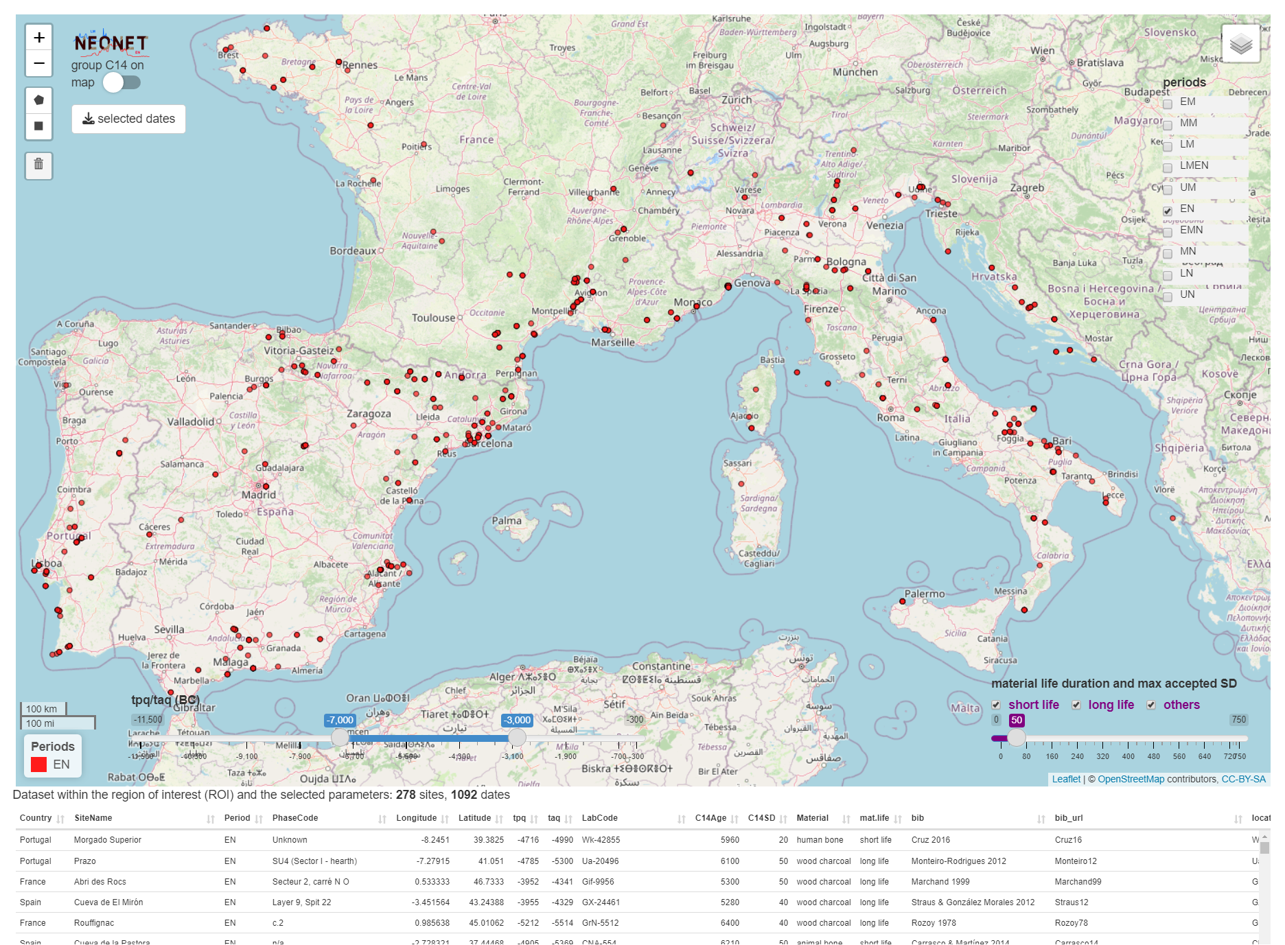
Screen capture of the NeoNet app before the export of the `neonet-data-2023-09-24.geojson` file: Early Neolithic (EN) dates only having a SD ≤ 50, and calBC interval between -7000 and -3000
The output is a map with isochrones calculated on the median of calibrated dates.
library(rcarbon)

source("R/neo_isochr.R")
source("R/neo_spd.R")
source("R/neo_calib.R")

neo_isochr(df.c14 = "https://raw.githubusercontent.com/zoometh/neonet/main/results/neonet-data-2023-09-24.geojson",
           show.lbl = FALSE)
Where neo_calib() calculate the cal BC min and max (i.e, calibrates), and the medidan (with 'intcal20' and the Bchron R package)
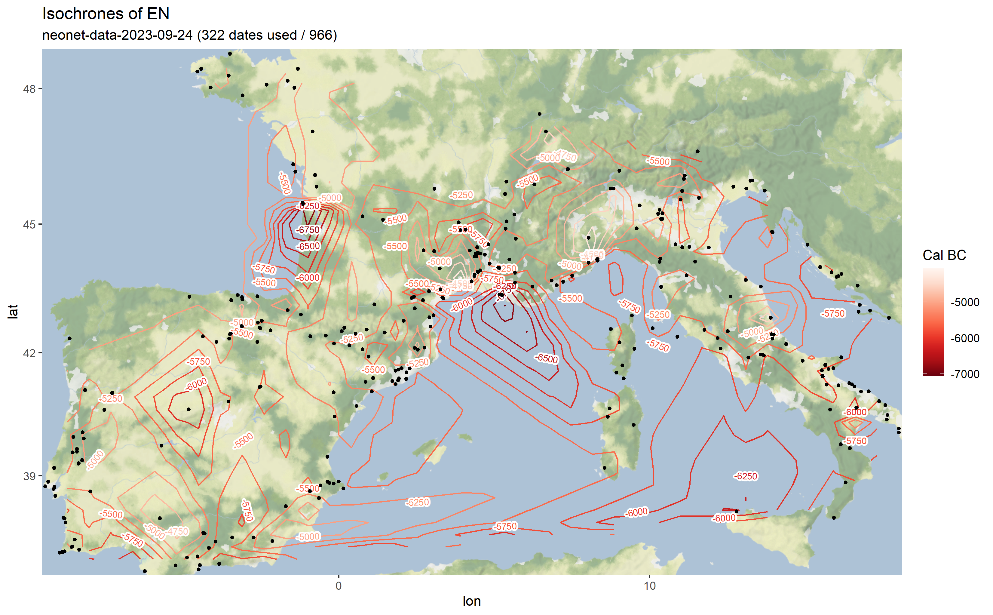
Output map from the `neonet-data-2023-09-24.geojson`
The same function can be used symetrically: instead of plotting the earliest dates of the Neolithic, one can also plot the latest dates of the Paleolithic
myc14data <- "https://raw.githubusercontent.com/zoometh/neonet/main/results/1_AOI_France_E-W.geojson"
neo_isochr(df.c14 = myc14data, mapname = "France_EW")
neo_isochr(df.c14 = myc14data, mapname = "France_EW", selected.per = c("LM"))
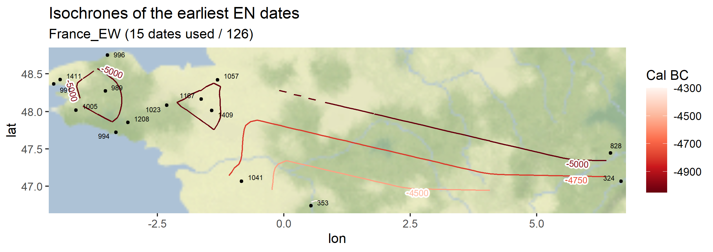
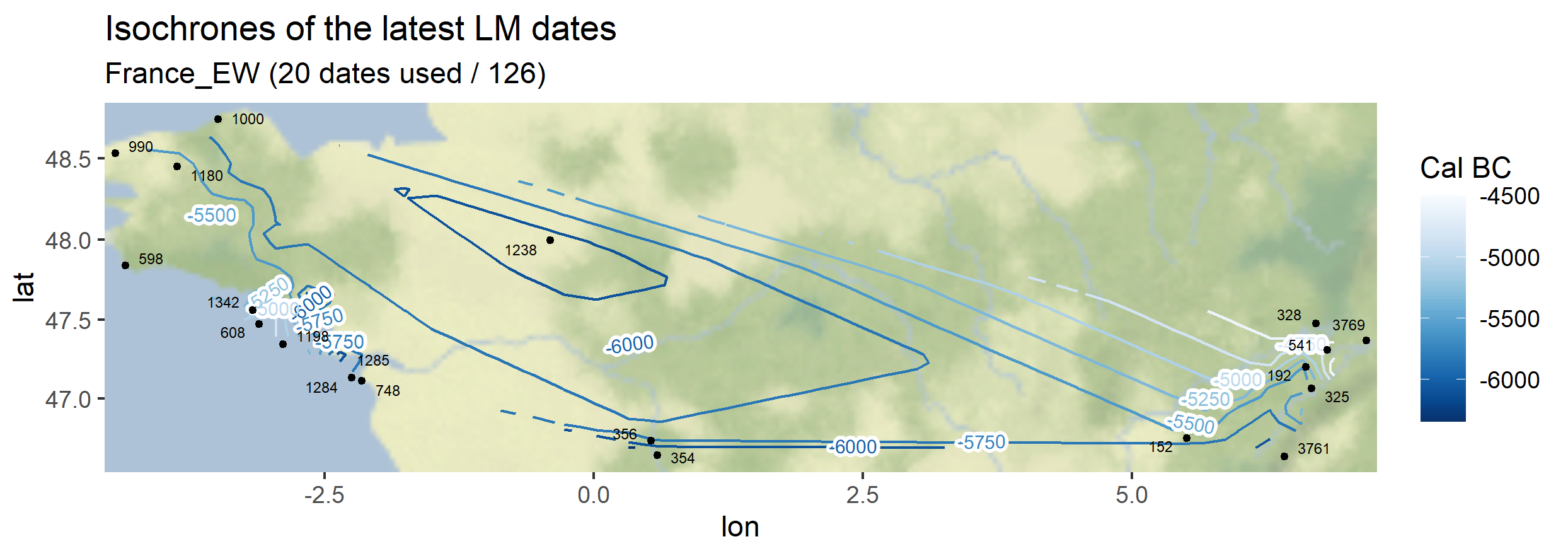
Output maps from the `1_AOI_France_E-W.geojson`: earliest Neolithic dates and latest Paleolithic dates
KCC, Koppen Climate Classification, Koeppen Climate Classification
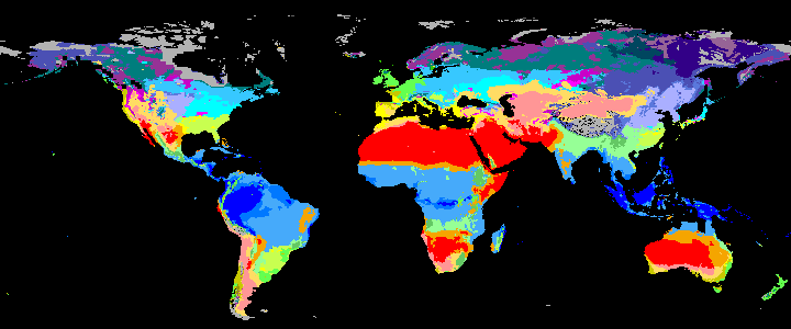
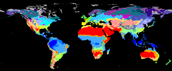
The app integrates Koppen Climate Classification (KCC) for 6,000 BP to 10,000 BP created with the R pastclim package and the neo_kcc_create() function.
The Koppen Climate Classification calculated for 8,000 BP (8k) with the pastclim R package and hosted on a GeoServer
Neonet functions help to blend pastclim KCC and radiocarbon dates.
# install the packages pastclim and terra
devtools::install_github("EvolEcolGroup/pastclim", ref="dev")
library(pastclim)
library(terra)

# set paths and create maps
outDir <- "C:/Rprojects/neonet/doc/data/clim/"
pastclim::set_data_path(path_to_nc = outDir)

source("R/neo_kcc_create.R")
neo_kcc_create()
Creates these KCC GeoTiffs:
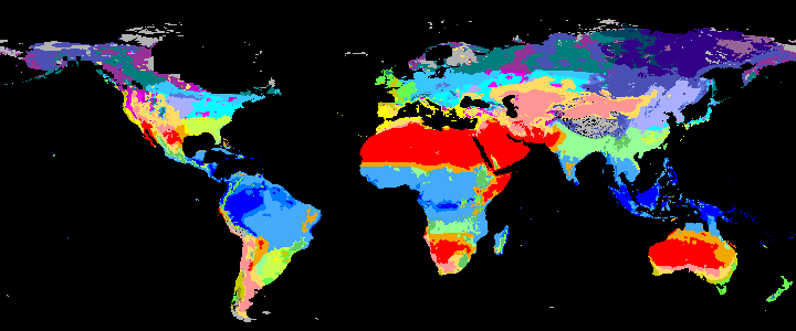
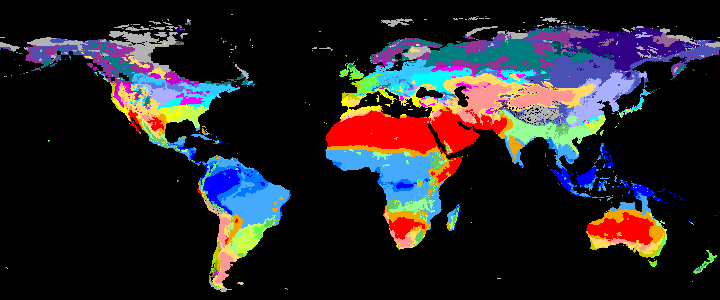
KCC are created as GeoTiffs using the R pastclim package
| Geotiff image | description |
|---|---|
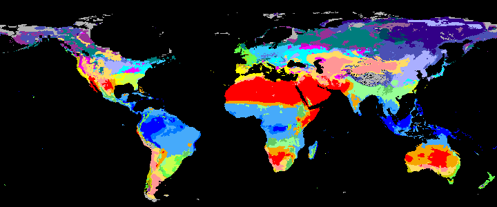 |
koppen_11k |
 |
koppen_10k |
 |
koppen_9k |
 |
koppen_8k |
 |
koppen_7k |
|
koppen_6k |
Past Koppen Climate Classification calculated in Kyears BP with the pastclim R package
The Koppen Climate Classes are listed here
| code | num | value | hexa color | color |
|---|---|---|---|---|
| Af | 1 | Tropical, rainforest | 0000FF |  |
| Am | 2 | Tropical, monsoon | 0078FF |  |
| Aw | 3 | Tropical, savannah | 46AAF |  |
| BWh | 4 | Arid, desert, hot | FF0000 |  |
| BWk | 5 | Arid, desert, cold | FF9696 |  |
| BSh | 6 | Arid, steppe, hot | F5A500 |  |
| BSk | 7 | Arid, steppe, cold | FFDC64 |  |
| Csa | 8 | Temperate, dry summer, hot summer | FFFF00 |  |
| Csb | 9 | Temperate, dry summer, warm summer | C8C800 |  |
| Csc | 10 | Temperate, dry summer, cold summer | 969600 |  |
| Cwa | 11 | Temperate, dry winter, hot summer | 96FF96 |  |
| Cwb | 12 | Temperate, dry winter, warm summer | 64C864 |  |
| Cwc | 13 | Temperate, dry winter, cold summer | 329632 |  |
| Cfa | 14 | Temperate, no dry season, hot summer | C8FF50 |  |
| Cfb | 15 | Temperate, no dry season, warm summer | 64FF50 |  |
| Cfc | 16 | Temperate, no dry season, cold summer | 32C800 |  |
| Dsa | 17 | Cold, dry summer, hot summer | FF00FF |  |
| Dsb | 18 | Cold, dry summer, warm summer | C800C8 |  |
| Dsc | 19 | Cold, dry summer, cold summer | 963296 |  |
| Dsd | 20 | Cold, dry summer, very cold winter | 966496 |  |
| Dwa | 21 | Cold, dry winter, hot summer | AAAF |  |
| Dwb | 22 | Cold, dry winter, warm summer | 5A78DC |  |
| Dwc | 23 | Cold, dry winter, cold summer | 4B50B4 |  |
| Dwd | 24 | Cold, dry winter, very cold winter | 320087 |  |
| Dfa | 25 | Cold, no dry season, hot summer | 00FFFF |  |
| Dfb | 26 | Cold, no dry season, warm summer | 37C8FF |  |
| Dfc | 27 | Cold, no dry season, cold summer | 007D7D |  |
| Dfd | 28 | Cold, no dry season, very cold winter | 00465F |  |
| ET | 29 | Polar, tundra | B2B2B2 |  |
| EF | 30 | Polar, frost | 666666 |  |
Koppen functions are designed not only for the Neonet dataset, but also for all radiocarbon dataset respecting the minimum data stracture (site, labcode, x, y, etc.).
The neo_kcc_map() creates a KCC map with a layer of dates above
source("R/config.R") # default variables: column names mapping, colors, etc.
df <- c14bazAAR::get_c14data("neonet")
df <- sf::st_as_sf(df, coords = c("lon", "lat"), crs = 4326)
neo_kcc_map(df.c14 = df,
kcc = "C:/Rprojects/neonet/doc/data/clim/koppen_7k.tif",
export = TRUE,
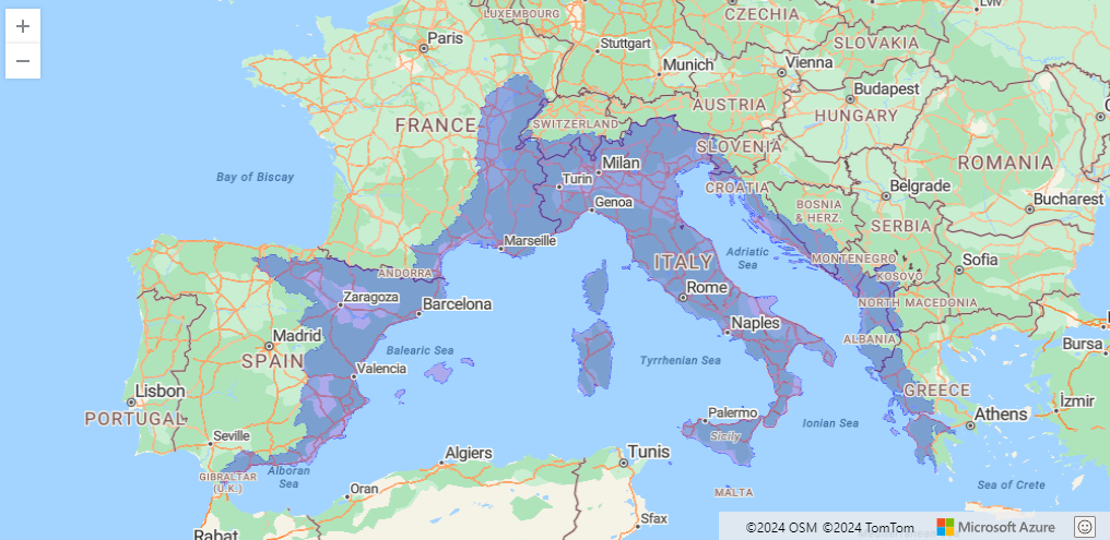
fileOut = "neonet_kcc.png" )Gives:
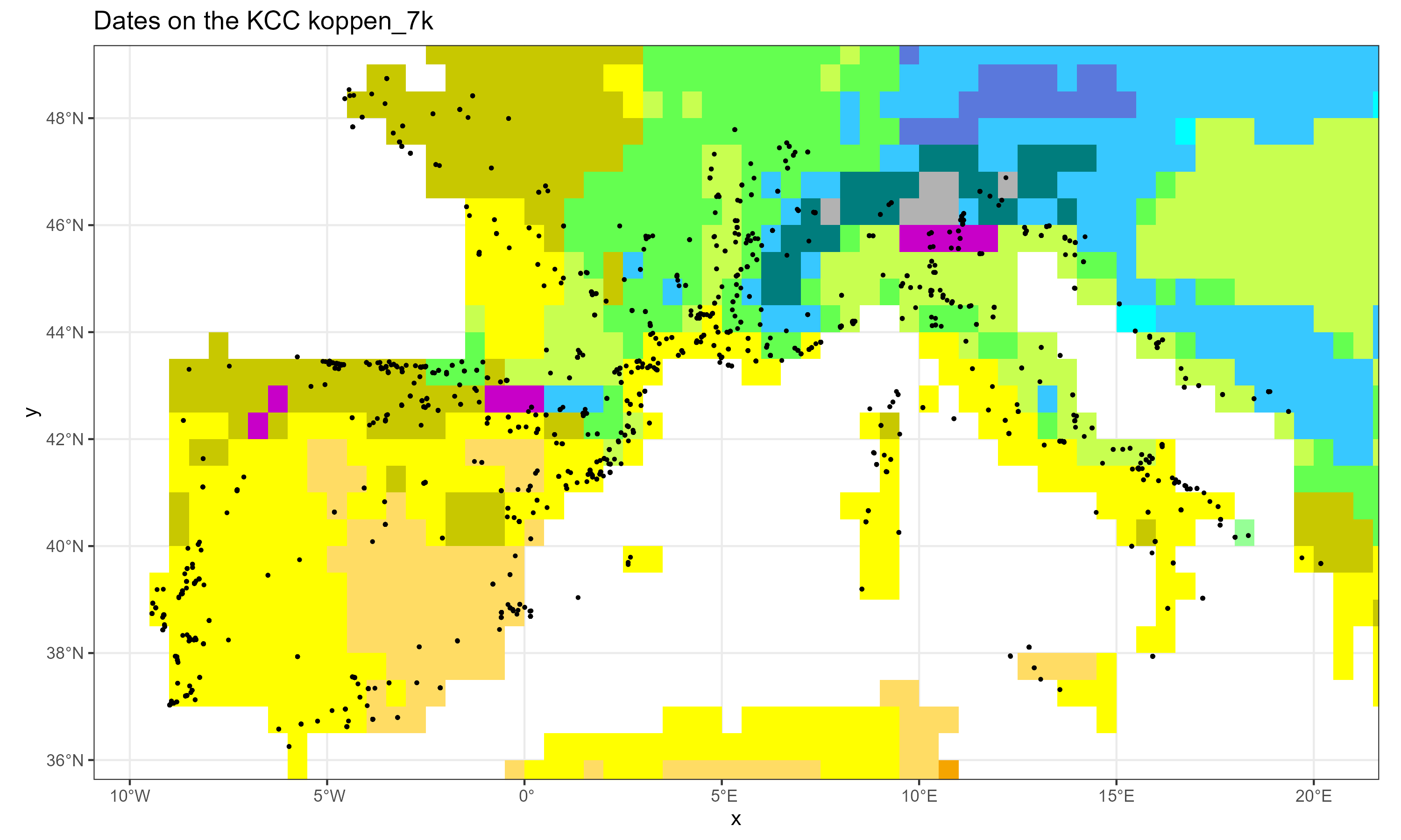
The neonet dataset over the KCC 7k
Or:
To assess what were the climates classes that where inhabited in the past, during the Late Mesolithic (LM) and Middle Mesolithic (MM) based on previous dates
df.c14 <- neo_calib(df.c14)
df.c14 <- sf::st_as_sf(df.c14, coords = c("lon", "lat"), crs = 4326)
kcc.file <- c("koppen_6k.tif", "koppen_7k.tif", "koppen_8k.tif",
              "koppen_9k.tif", "koppen_10k.tif", "koppen_11k.tif")
df_cc <- neo_kcc_extract(df.c14 = df.c14, kcc.file = kcc.file)
col.req <- gsub(pattern = ".tif", "", kcc.file)
neo_kcc_plotbar(df_cc = df_cc,
                kcc.file = c("koppen_8k.tif", "koppen_9k.tif"),
                col.req = col.req,
                selected.per = c("EN"),
                title = "Neolithic: transition btw 7,000 and 6,000 BC",
                legend.show = FALSE)
Gives:
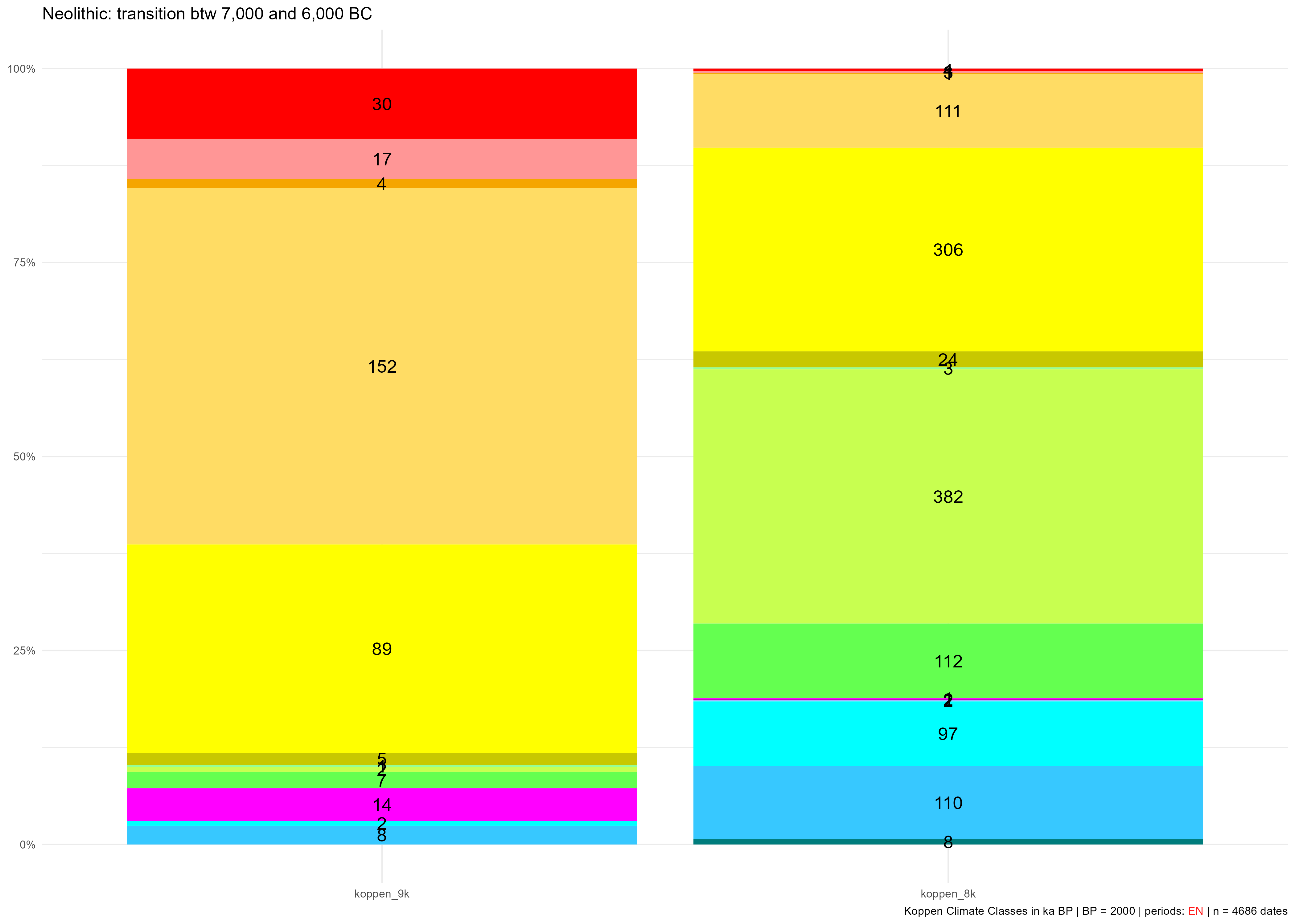
KCC occupied during the EN between 7,000 and 6,000 BC (9 ka and 8 ka BP) with counts of sites belonging to these time slices
The neo_kcc_extract() function collects the KCC values (climates) of each date.
NeoNet-strati is an online R Shiny interactive app to record the stratigraphy of NeoNet's archaeological sites in an editable dataframe based on LabCode identifiers.
flowchart TD
    A[NeoNet dataset] --is read by--> B{{<a href='https://trainingidn.shinyapps.io/neonet-strati'>neonet-strati</a>}}:::neonetshiny;
    B --edit<br>site stratigraphy--> B;
    B --export<br>site stratigraphy<br>file--> C[<a href='https://github.com/historical-time/data-samples/blob/main/neonet/Roc%20du%20Dourgne_2023-07-30.csv'>Roc du Dourgne_2023-07-30.csv</a>];
    C --is read by--> D{{<a href='https://github.com/historical-time/caa23/blob/main/neonet/functions/neo_strat.R'>neonet_strat</a>}}:::neonetfunct;
    D --export --> E[maps<br>charts<br>listings<br>...];
    classDef neonetfunct fill:#e3c071;
    classDef neonetshiny fill:#71e37c;
Strati app and strati analysis overall Workflow
The app is composed by different panels: a site to be recorded (Site Stratigraphy panel), and the complete dataset (All sites panel). A site name is copied from All sites panel to Site Stratigraphy panel.
Plot a selected site in an editable table to record its stratigraphical relationships.
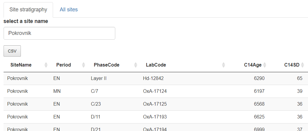
Panel "Site Stratigraphy" editable dataframe. By default the app opens on "Pokrovnik"
Show the complete NeoNet dataset. A site can be selected by searching it in the selection search bar (top-right) and copying its name (Site Name column). Here Roc du Dourgne, highlighted in blue.
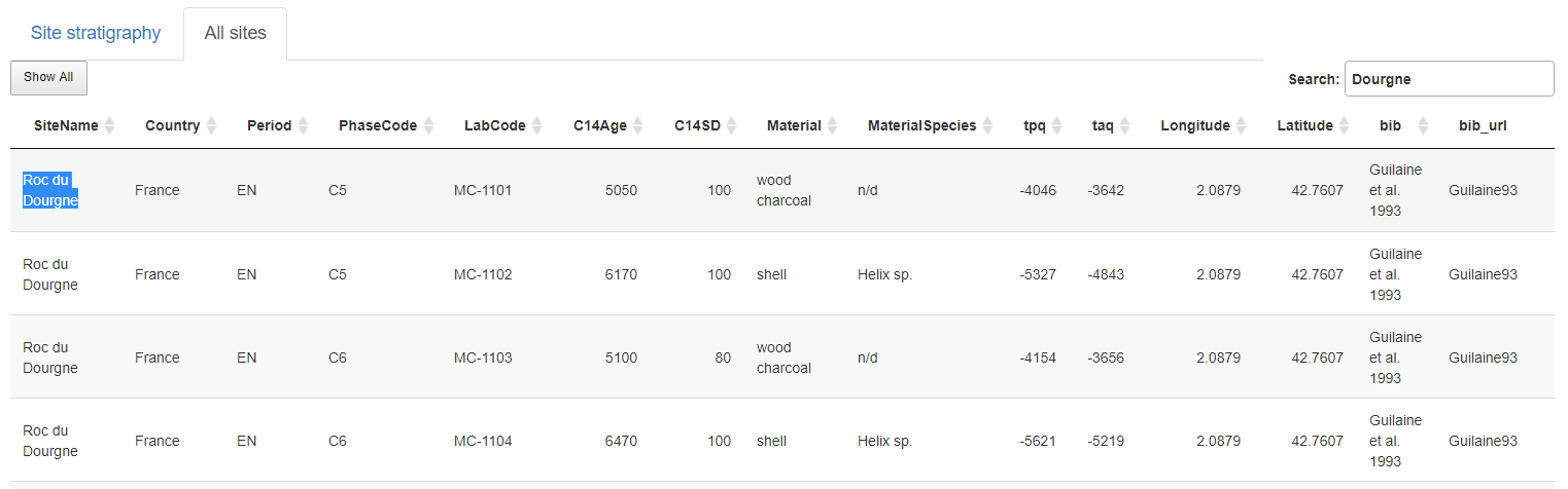
Panel "All sites". Selection of the "Roc du Dourgne" site
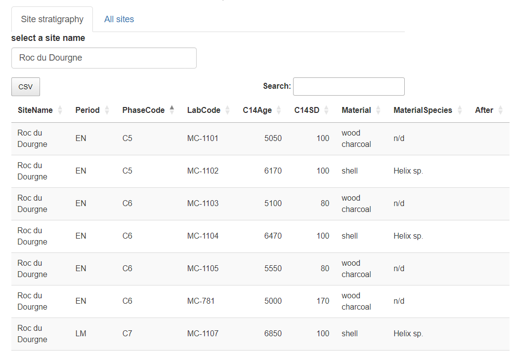
"Roc du Dourgne" site sorted on its "PhaseCode"
The stratigraphical relations can be added into the "After" column, and thereafter exported in CSV
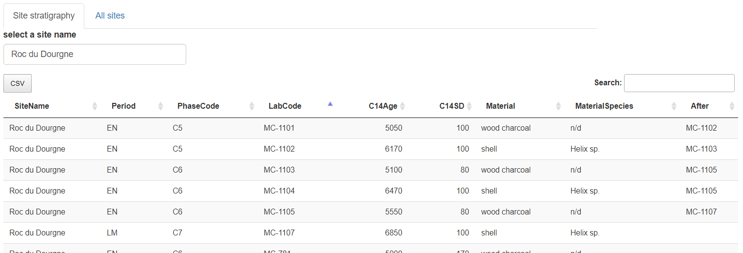
"Roc du Dourgne" stratgraphical relationships (column "After") after edition
For example, "Roc du Dourgne" relationships are:
| LabCode | After | Period | PhaseCode | C14Age | C14SD |
|---|---|---|---|---|---|
| MC-1101 | MC-1102 | EN | C5 | 5050 | 100 |
| MC-1102 | MC-1103 | EN | C5 | 6170 | 100 |
| MC-1103 | MC-1105 | EN | C6 | 5100 | 80 |
| MC-1104 | MC-1105 | EN | C6 | 6470 | 100 |
| MC-1105 | MC-1107 | EN | C6 | 5550 | 80 |
| MC-1107 | LM | C7 | 6850 | 100 | |
| MC-781 | EN | C6 | 5000 | 170 | |
| MC-782 | LM | Layer 7 | 5770 | 170 |
The first row can be read as: "the layer containing radiocarbon date MC-1101 comes after the layer containing radiocarbon date MC-1102".
Once the site stratigraphy recorded, save the changes by downloading the dataset pressing the button (top-left) as a CSV file. The output file name is the site name and the current date (ex: Roc du Dourgne_2024-04-12.csv).
The file exported from the NeoNet strati app can be read by the neo_strati() function (see Harris Matrix)
The output CSV file exported by NeoNet-strati can be read by the neo_strat() function. For example, ploting the C14Age and the PhaseCode.
neo_strat(inData = 'https://raw.githubusercontent.com/historical-time/data-samples/main/neonet/Roc du Dourgne_2023-07-30.csv',
          outLabel = c("C14Age"))
neo_strat(inData = 'https://raw.githubusercontent.com/historical-time/data-samples/main/neonet/Roc du Dourgne_2023-07-30.csv',
          outLabel = c("PhaseCode"))
Gives:
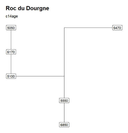
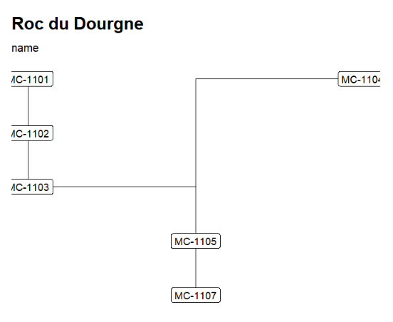
"Roc du Dourgne" stratgraphical relationships using LabCode identifiers, ordered on the "LabCode" column, displaying the C14Age (left) and the LabCode (right)
Changing the outLabel to Period allows to color on periods using the default period colors (see the web document)
neo_strat(inData = 'https://raw.githubusercontent.com/historical-time/data-samples/main/neonet/Roc du Dourgne_2023-07-30.csv',
          outLabel = c("Period"))
Gives:
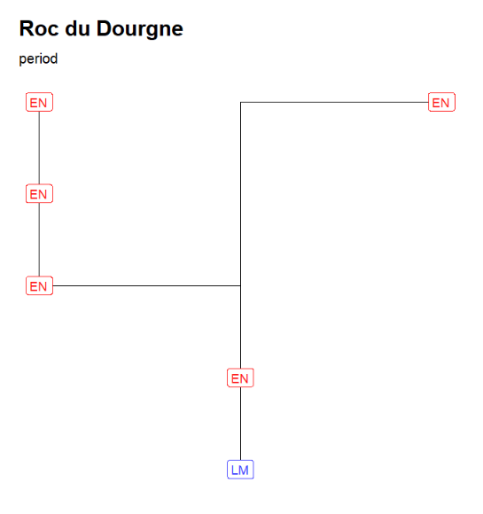
"Roc du Dourgne" stratgraphical relationships using LabCode identifiers, ordered on the "LabCode" column
Using neo_leapfrog(DT = T) to merge dataframe from NeoNet and Leapfrog on common C14 LabCode values: https://historical-time.github.io/caa23/neonet/results/NN_and_LF.html

Screen capture of [NN_and_LF.html](https://historical-time.github.io/caa23/neonet/results/NN_and_LF.html)
- NeoNet app web document
- Contribution rules
- NeoNet package license
- Big Historical Data Conference
- Shiny server (with the app embeded): http://shinyserver.cfs.unipi.it:3838/neonet/bhdc
- GitHub (without the app embeded): https://zoometh.github.io/neonet/doc/talks/2023-bhdc
- Neonet workshop
- SIMEP