NeuralPDE

NeuralPDE.jl is a solver package which consists of neural network solvers for partial differential equations using scientific machine learning (SciML) techniques such as physics-informed neural networks (PINNs) and deep BSDE solvers. This package utilizes deep neural networks and neural stochastic differential equations to solve high-dimensional PDEs at a greatly reduced cost and greatly increased generality compared with classical methods.

Installation

Assuming that you already have Julia correctly installed, it suffices to install NeuralPDE.jl in the standard way, that is, by typing ] add NeuralPDE. Note: to exit the Pkg REPL-mode, just press Backspace or Ctrl + C.

Tutorials and Documentation

For information on using the package, see the stable documentation. Use the in-development documentation for the version of the documentation, which contains the unreleased features.

Features

Physics-Informed Neural Networks for automated PDE solving
Forward-Backwards Stochastic Differential Equation (FBSDE) methods for parabolic PDEs
Deep-learning-based solvers for optimal stopping time and Kolmogorov backwards equations

Example: Solving 2D Poisson Equation via Physics-Informed Neural Networks

using NeuralPDE, Flux, ModelingToolkit, GalacticOptim, Optim, DiffEqFlux

@parameters x y
@variables u(..)
Dxx = Differential(x)^2
Dyy = Differential(y)^2

# 2D PDE
eq  = Dxx(u(x,y)) + Dyy(u(x,y)) ~ -sin(pi*x)*sin(pi*y)

# Boundary conditions
bcs = [u(0,y) ~ 0.f0, u(1,y) ~ -sin(pi*1)*sin(pi*y),
       u(x,0) ~ 0.f0, u(x,1) ~ -sin(pi*x)*sin(pi*1)]
# Space and time domains
domains = [x ∈ IntervalDomain(0.0,1.0),
           y ∈ IntervalDomain(0.0,1.0)]
# Discretization
dx = 0.1

# Neural network
dim = 2 # number of dimensions
chain = FastChain(FastDense(dim,16,Flux.σ),FastDense(16,16,Flux.σ),FastDense(16,1))

discretization = PhysicsInformedNN(chain, GridTraining(dx))

pde_system = PDESystem(eq,bcs,domains,[x,y],[u])
prob = discretize(pde_system,discretization)

cb = function (p,l)
    println("Current loss is: $l")
    return false
end

res = GalacticOptim.solve(prob, Optim.BFGS(); cb = cb, maxiters=1000)
phi = discretization.phi

And some analysis:

xs,ys = [domain.domain.lower:dx/10:domain.domain.upper for domain in domains]
analytic_sol_func(x,y) = (sin(pi*x)*sin(pi*y))/(2pi^2)

u_predict = reshape([first(phi([x,y],res.minimizer)) for x in xs for y in ys],(length(xs),length(ys)))
u_real = reshape([analytic_sol_func(x,y) for x in xs for y in ys], (length(xs),length(ys)))
diff_u = abs.(u_predict .- u_real)

using Plots
p1 = plot(xs, ys, u_real, linetype=:contourf,title = "analytic");
p2 = plot(xs, ys, u_predict, linetype=:contourf,title = "predict");
p3 = plot(xs, ys, diff_u,linetype=:contourf,title = "error");
plot(p1,p2,p3)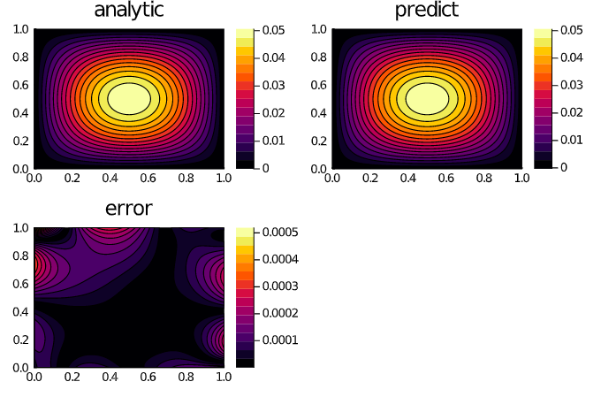

Example: Solving a 100-Dimensional Hamilton-Jacobi-Bellman Equation

using NeuralPDE
using Flux
using DifferentialEquations
using LinearAlgebra
d = 100 # number of dimensions
X0 = fill(0.0f0, d) # initial value of stochastic control process
tspan = (0.0f0, 1.0f0)
λ = 1.0f0

g(X) = log(0.5f0 + 0.5f0 * sum(X.^2))
f(X,u,σᵀ∇u,p,t) = -λ * sum(σᵀ∇u.^2)
μ_f(X,p,t) = zero(X)  # Vector d x 1 λ
σ_f(X,p,t) = Diagonal(sqrt(2.0f0) * ones(Float32, d)) # Matrix d x d
prob = TerminalPDEProblem(g, f, μ_f, σ_f, X0, tspan)
hls = 10 + d # hidden layer size
opt = Flux.ADAM(0.01)  # optimizer
# sub-neural network approximating solutions at the desired point
u0 = Flux.Chain(Dense(d, hls, relu),
                Dense(hls, hls, relu),
                Dense(hls, 1))
# sub-neural network approximating the spatial gradients at time point
σᵀ∇u = Flux.Chain(Dense(d + 1, hls, relu),
                  Dense(hls, hls, relu),
                  Dense(hls, hls, relu),
                  Dense(hls, d))
pdealg = NNPDENS(u0, σᵀ∇u, opt=opt)
@time ans = solve(prob, pdealg, verbose=true, maxiters=100, trajectories=100,
                            alg=EM(), dt=1.2, pabstol=1f-2)

zoemcc / NeuralPDE.jl