The purpose of the package are to help analysis the LI-6800 induction data with JIP test,The method of calculation are from:
Tsimilli-michael M. Revisiting JIP-test: Aneducative review on concepts, assumptions, approximations, definitions and terminology[J].Photosynthetica,2019,57 (SI): 90-107.
As I am not a scientist, so please use with caution, and check the
jip_comp.R for the calculations. Any feedback will be appreciated.
What I am sure to help is the plot method to help view the data
quickly.
To install:
devtools::install_github("zhujiedong/jiptest")To load:
library(jiptest)There are 2 functions for this purpose, one is read_induction, it is
meant to read a single induction excel file:
# list all the induction excel files here
files <- list.files("inst/extdata/ojip", full.names = TRUE)
ojip_file1 <- read_induction(files[1])

knitr::kable(head(ojip_file1[,1:4]))| EVENT_ID | TRACE_NO | SECS | FLUOR |
|---|---|---|---|
| MARGIN | 5 | 1.90e-06 | 971 |
| DURATION | 1000 | 6.00e-06 | 971 |
| Q_RED_SETPOINT | 15000 | 1.00e-05 | 1002 |
| D_RED_PERCENT | 90 | 1.41e-05 | 1118 |
| FMAX | 3390.12 | 1.81e-05 | 1185 |
| QMAX | 15481.4 | 2.19e-05 | 1071 |
Another one is a wrap of read_induction, just help to read all excel
data in a folder, and in a so called tidy data form:
all_files <- read_all_induction("inst/extdata/ojip")## New names:
## New names:
## New names:
## New names:
## New names:
## New names:
## • `` -> `...1`
## • `` -> `...2`
## • `` -> `...3`
## • `` -> `...4`
## • `` -> `...5`
## • `` -> `...6`
## • `` -> `...7`
## • `` -> `...8`
## • `` -> `...9`
knitr::kable(rbind(head(all_files), tail(all_files)))| EVENT_ID | TRACE_NO | SECS | FLUOR | DC | PFD | REDMODAVG | CODE | SOURCE | NORM_FLUOR | NORM_DC | MILLI_SEC |
|---|---|---|---|---|---|---|---|---|---|---|---|
| MARGIN | 5 | 0.0000019 | 971.00 | 163589 | 15474.2 | 24.9990 | 3 | INDUCTION-26-20201026-16_07_50 | 0.0000000 | 0.0000000 | 1.90740e-03 |
| DURATION | 1000 | 0.0000060 | 971.00 | 166127 | 15468.7 | 24.9990 | 3 | INDUCTION-26-20201026-16_07_50 | 0.0000000 | 0.0071962 | 5.96060e-03 |
| Q_RED_SETPOINT | 15000 | 0.0000100 | 1002.00 | 168725 | 15468.3 | 24.9990 | 3 | INDUCTION-26-20201026-16_07_50 | 0.0128031 | 0.0145625 | 1.00137e-02 |
| D_RED_PERCENT | 90 | 0.0000141 | 1118.00 | 171303 | 15467.2 | 24.9990 | 3 | INDUCTION-26-20201026-16_07_50 | 0.0607117 | 0.0218721 | 1.40668e-02 |
| FMAX | 3390.12 | 0.0000181 | 1185.00 | 174013 | 15468.2 | 24.9990 | 3 | INDUCTION-26-20201026-16_07_50 | 0.0883830 | 0.0295560 | 1.81198e-02 |
| QMAX | 15481.4 | 0.0000219 | 1071.00 | 176819 | 15468.6 | 24.9990 | 3 | INDUCTION-26-20201026-16_07_50 | 0.0413005 | 0.0375121 | 2.19346e-02 |
| NA | NA | 0.9800160 | 4129.87 | 635389 | 15117.4 | 24.9986 | 3 | INDUCTION-486-20171225-14_33_46 | 0.9706033 | 0.9751675 | 9.80016e+02 |
| NA | NA | 0.9840160 | 4132.01 | 635327 | 15117.3 | 24.9986 | 3 | INDUCTION-486-20171225-14_33_46 | 0.9712629 | 0.9750420 | 9.84016e+02 |
| NA | NA | 0.9880160 | 4127.78 | 635262 | 15117.1 | 24.9986 | 3 | INDUCTION-486-20171225-14_33_46 | 0.9699591 | 0.9749105 | 9.88016e+02 |
| NA | NA | 0.9920160 | 4126.07 | 635200 | 15117.0 | 24.9986 | 3 | INDUCTION-486-20171225-14_33_46 | 0.9694320 | 0.9747850 | 9.92016e+02 |
| NA | NA | 0.9960160 | 4127.87 | 635136 | 15116.9 | 24.9986 | 3 | INDUCTION-486-20171225-14_33_46 | 0.9699868 | 0.9746555 | 9.96016e+02 |
| NA | NA | 1.0000200 | 4125.81 | 635077 | 15108.1 | 24.9986 | 3 | INDUCTION-486-20171225-14_33_46 | 0.9693518 | 0.9745361 | 1.00002e+03 |
The calculation is done by jip_test function, it has a parameter
called use_PAM, the default value is FALSE, which means it will use
the DC (continuous fluorescence) data by default (recomended as it has
high signal/noise ratio), else it will use the AC (PAM) fluorescence.
ojip_data_pam <- jip_test(ojip_file1, use_PAM = TRUE)
ojip_data<- jip_test(ojip_file1)
knitr::kable(tail(ojip_data))| OJIP_PARAMETERS | VALUES | SOURCE |
|---|---|---|
| Sm | 1.080540e+00 | INDUCTION-26-20201026-16_07_50 |
| N | 1.411901e+06 | INDUCTION-26-20201026-16_07_50 |
| RC_ABS | 5.000000e-07 | INDUCTION-26-20201026-16_07_50 |
| gamma_RC | 5.000000e-07 | INDUCTION-26-20201026-16_07_50 |
| PI_ABS | 9.000000e-07 | INDUCTION-26-20201026-16_07_50 |
| PI_total | 3.000000e-07 | INDUCTION-26-20201026-16_07_50 |
There is a column called SOURCE, which use the file name of each excel
file to distinguish where these data come from.
all_data_continuous<- jip_test(all_files)
all_data_pam <- jip_test(all_files, use_PAM = TRUE)
For most normalized calculated parameters, the differences between use_PAM or not are almost zero:
cat(sprintf("difference value of %s are:\n %.3f\n", ojip_data$OJIP_PARAMETERS, ojip_data$VALUES - ojip_data_pam$VALUES))## difference value of F20us are:
## 172828.000
## difference value of F50us are:
## 194769.000
## difference value of F100us are:
## 226884.000
## difference value of F300us are:
## 300152.000
## difference value of FJ are:
## 352927.200
## difference value of FI are:
## 473990.170
## difference value of FP are:
## 512882.720
## difference value of Area are:
## 365800.722
## difference value of FO are:
## 172828.000
## difference value of FM are:
## 512882.720
## difference value of FV are:
## 340054.720
## difference value of VJ are:
## 0.010
## difference value of VI are:
## 0.012
## difference value of MO are:
## 687656.186
## difference value of Ss are:
## -0.000
## difference value of phi_Po are:
## 0.012
## difference value of phi_Eo are:
## -0.001
## difference value of phi_Ro are:
## -0.006
## difference value of Psi_Eo are:
## -0.010
## difference value of delta_Ro are:
## -0.019
## difference value of ABS_RC are:
## 1958302.410
## difference value of TRo_RC are:
## 1298402.787
## difference value of ETo_RC are:
## 610746.601
## difference value of REo_RC are:
## 148502.170
## difference value of ECo_RC are:
## -0.744
## difference value of Sm are:
## -0.744
## difference value of N are:
## 1396831.593
## difference value of RC_ABS are:
## -0.000
## difference value of gamma_RC are:
## -0.000
## difference value of PI_ABS are:
## -0.000
## difference value of PI_total are:
## -0.000
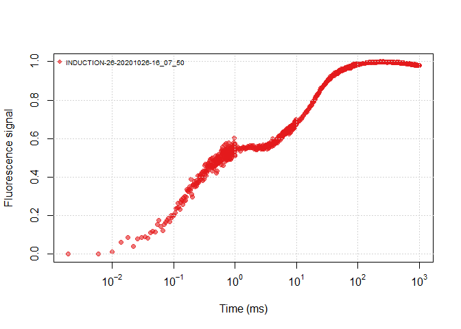
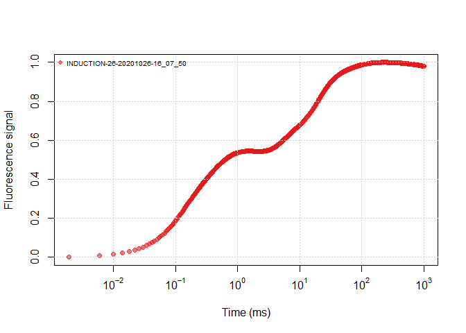
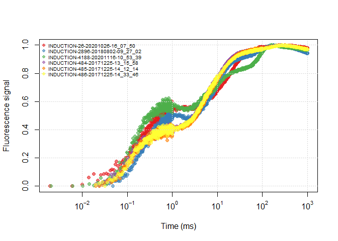
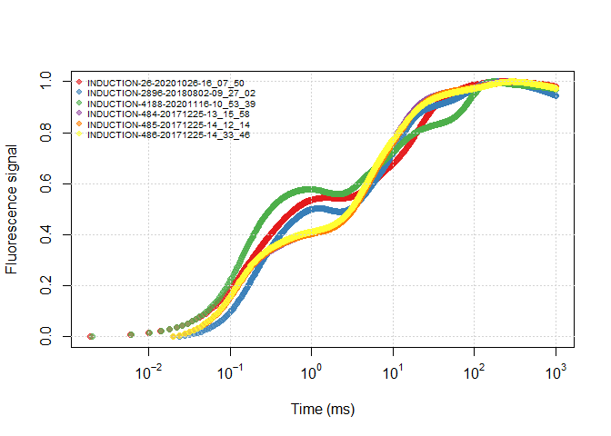
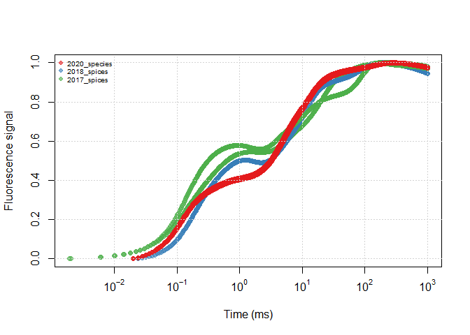
It is helpful to view all the data through a plot, you can view an OJIP plot by the following ways:
plot(ojip_file1, use_PAM = TRUE)plot(ojip_file1)plot(all_files, use_PAM = TRUE)plot(all_files)Similar to other functions with argument use_PAM, you can view the PAM
data or the continuous data. The fluorecence data are normalized by:
it will help the Y axis in a range of 0~1.
Assume my example data (these excel file in the folder of ojip) contains
flies of different treatments (actually they belong to different species
that test in different years), we assume data from the same year
(indicated by the file names) are the same treatment. we should change
the column of SOURCE in the data file to assign what treatment they
really belongs to, to substitute the excel file names when they are
imported:
First we should check the file names of SOURCE:
unique(all_files$SOURCE)## [1] "INDUCTION-26-20201026-16_07_50" "INDUCTION-2896-20180802-09_27_02"
## [3] "INDUCTION-4188-20201116-10_53_39" "INDUCTION-484-20171225-13_15_58"
## [5] "INDUCTION-485-20171225-14_12_14" "INDUCTION-486-20171225-14_33_46"
Then we can use a function from jiptest called sub_name to help
change the SOURCE column to different groups that indicate
treatments/replications etc.
# use a short name that easy to distinguish
rep_all <-
  c('2020_species',
    '2018_spices',
    '2020_species',
    rep('2017_spices', 3))
df <- all_files
df$SOURCE <- sub_name(df, rep_all)plot(all_files)plot(df)It is more clear to use the ‘real groups’ between data files to view differences between treatments/replications.
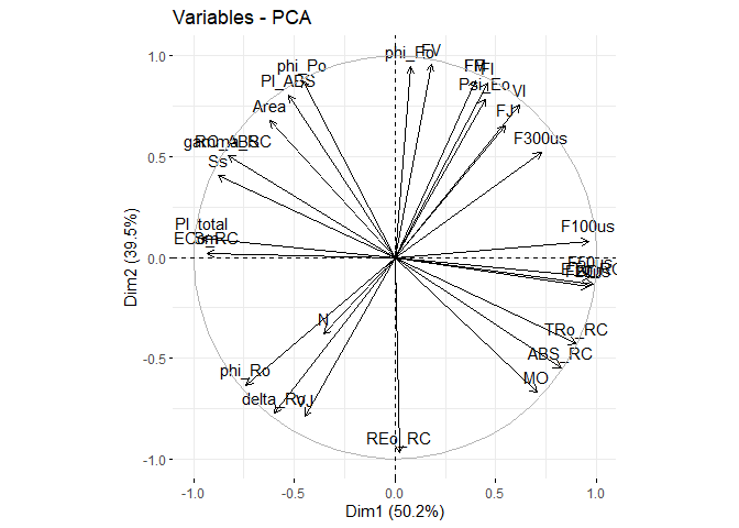
To help us analyse the results with PCA, a function called jip_pca can
help us to have a quick view of all the data. There is only one
parameter for the function, that is the returned data frame from
jiptest, to get the data for PCA analysis use continuous light:
library("FactoMineR")
library("factoextra")
## Loading required package: ggplot2
## Welcome! Want to learn more? See two factoextra-related books at https://goo.gl/ve3WBa
pca_df <- jip_pca(all_data_continuous)We can also use the same method to group the imported data from the excel files:
First we should check the file names of SOURCE (recommended in case
the wrong sequense happend):
pca_df$SOURCE## [1] "INDUCTION-26-20201026-16_07_50" "INDUCTION-2896-20180802-09_27_02"
## [3] "INDUCTION-4188-20201116-10_53_39" "INDUCTION-484-20171225-13_15_58"
## [5] "INDUCTION-485-20171225-14_12_14" "INDUCTION-486-20171225-14_33_46"
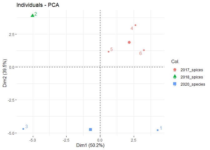
Then we can also use sun_name to help change the SOURCE column to
different groups that indicate treatments/replications etc.
# use a short name that easy to distinguish
treatment <-
  c('2020_species',
    '2018_spices',
    '2020_species',
    rep('2017_spices', 3))

pca_df$SOURCE <- sub_name(pca_df, treatment)
pca_df$SOURCE
## [1] "2020_species" "2018_spices" "2020_species" "2017_spices" "2017_spices"
## [6] "2017_spices"
df <- pca_df[,-1]
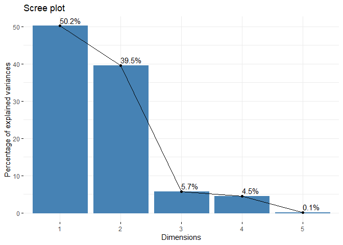
final_pca <- PCA(df, graph = FALSE)
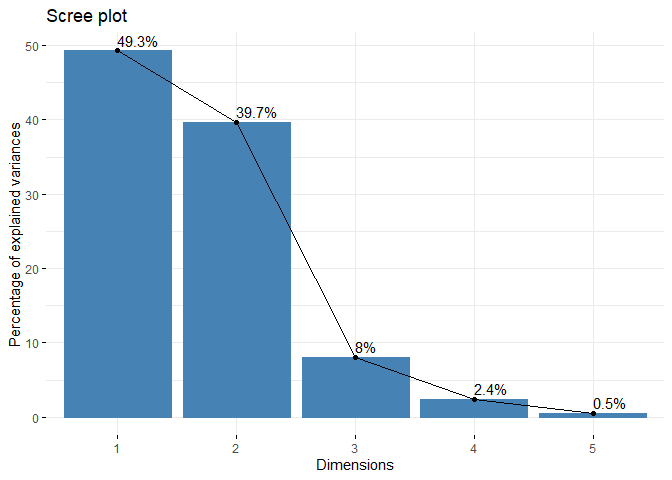
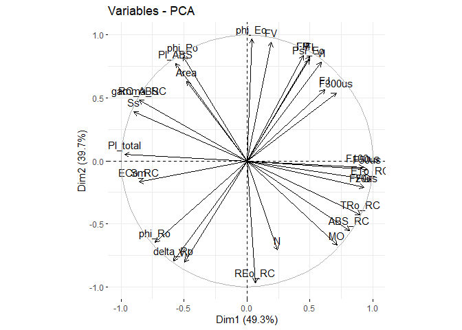
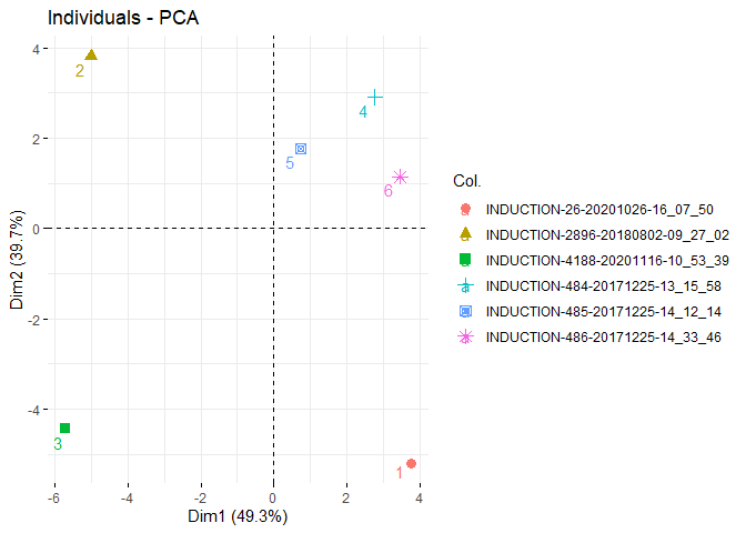
fviz_eig(final_pca, addlabels = TRUE)fviz_pca_var(final_pca)fviz_pca_ind(final_pca, repel = TRUE, col.ind= pca_df$SOURCE)To use PAM:
pca_df <- jip_pca(all_data_pam)

df <- pca_df[,-1]
final_pca <- PCA(df, graph = FALSE)
fviz_eig(final_pca, addlabels = TRUE)fviz_pca_var(final_pca)fviz_pca_ind(final_pca, repel = TRUE, col.ind= pca_df$SOURCE)