inspectdf is collection of utilities for columnwise summary,
comparison and visualisation of data frames. Functions are provided to
summarise missingness, categorical levels, numeric distribution,
correlation, column types and memory usage.
The package has three aims:
- to speed up repetitive checking and exploratory tasks for data frames
- to make it easier to compare data frames for differences and inconsistencies
- to support quick visualisation of data frames
inspect_types()summary of column typesinspect_mem()summary of memory usage of columnsinspect_na()columnwise prevalence of missing valuesinspect_cor()correlation coefficients of numeric columnsinspect_imb()feature imbalance of categorical columnsinspect_num()summaries of numeric columnsinspect_cat()summaries of categorical columns
To install the development version of the package, use
devtools::install_github("alastairrushworth/inspectdf")

# load the package
library(inspectdf)The examples below make use of the starwars data from the dplyr
package
# some example data
data(starwars, package = "dplyr")
For illustrating comparisons of dataframes, use the starwars data and
produce two new dataframes star_1 and star_2 that randomly sample
the rows of the original and drop a couple of columns.
library(dplyr)
star_1 <- starwars %>% sample_n(50)
star_2 <- starwars %>% sample_n(50) %>% select(-1, -2)To explore the column types in a data frame, use the function
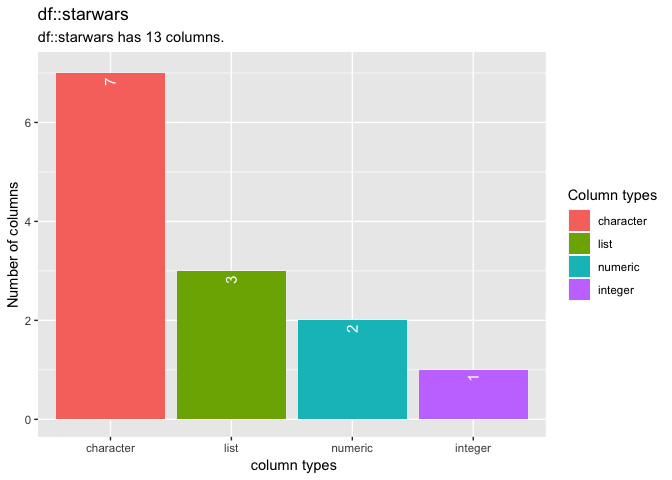
inspect_types(). The command returns a tibble summarising the counts
and percentages of columns with particular types. A barplot is also
returned when show_plot = TRUE.
# return tibble and visualisation of columns types
inspect_types(starwars, show_plot = TRUE)
## # A tibble: 4 x 4
## type cnt pcnt col_name
## <chr> <int> <dbl> <list>
## 1 character 7 53.8 <chr [7]>
## 2 list 3 23.1 <chr [3]>
## 3 numeric 2 15.4 <chr [2]>
## 4 integer 1 7.69 <chr [1]>
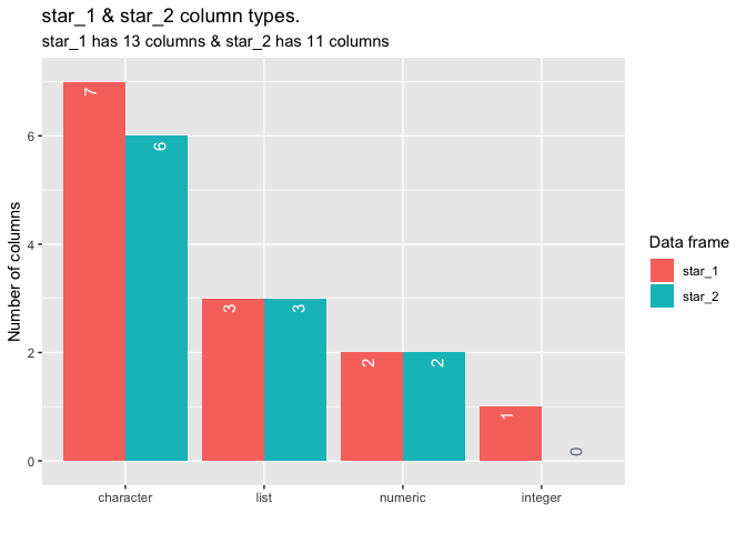
When a second dataframe is provided, inspect_types() will create a
dataframe comparing the count and percentage of each column type for
each of the input dataframes. The summaries for the first and second
dataframes are show in columns with names appended with _1 and _2,
respectively.
inspect_types(star_1, star_2, show_plot = TRUE)## # A tibble: 4 x 5
## type cnt_1 pcnt_1 cnt_2 pcnt_2
## <chr> <int> <dbl> <dbl> <dbl>
## 1 character 7 53.8 6 54.5
## 2 list 3 23.1 3 27.3
## 3 numeric 2 15.4 2 18.2
## 4 integer 1 7.69 0 0
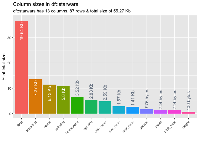
To explore the memory usage of the columns in a data frame, use
inspect_mem(). The command returns a tibble containing the size of
each column in the dataframe. A barplot is also returned when show_plot = TRUE.
inspect_mem(starwars, show_plot = TRUE)## # A tibble: 13 x 3
## col_name size pcnt
## <chr> <chr> <dbl>
## 1 films 19.54 Kb 36.5
## 2 starships 7.27 Kb 13.6
## 3 name 6.13 Kb 11.5
## 4 vehicles 5.8 Kb 10.8
## 5 homeworld 3.52 Kb 6.58
## 6 species 2.88 Kb 5.39
## 7 skin_color 2.59 Kb 4.85
## 8 eye_color 1.57 Kb 2.93
## 9 hair_color 1.41 Kb 2.63
## 10 gender 976 bytes 1.78
## 11 mass 744 bytes 1.36
## 12 birth_year 744 bytes 1.36
## 13 height 400 bytes 0.730
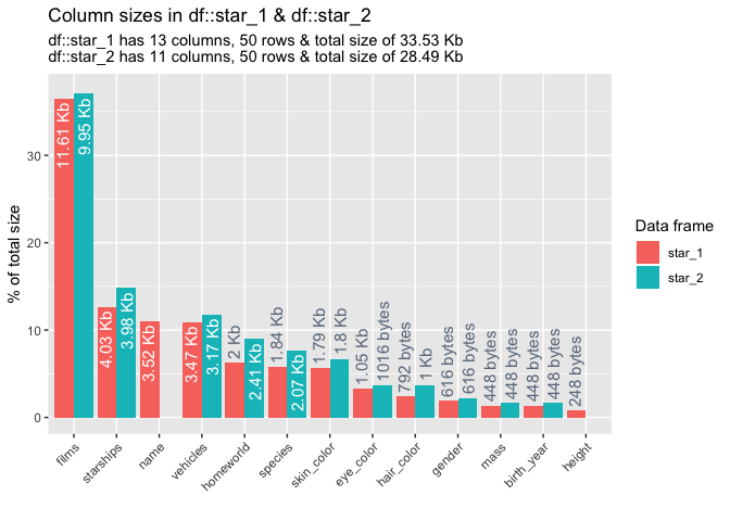
When a second dataframe is provided, inspect_mem() will create a
dataframe comparing the size of each column for both input dataframes.
The summaries for the first and second dataframes are show in columns
with names appended with _1 and _2, respectively.
inspect_mem(star_1, star_2, show_plot = TRUE)## # A tibble: 13 x 5
## col_name size_1 size_2 pcnt_1 pcnt_2
## <chr> <chr> <chr> <dbl> <dbl>
## 1 films 11.61 Kb 9.95 Kb 36.5 37.1
## 2 starships 4.03 Kb 3.98 Kb 12.7 14.8
## 3 name 3.52 Kb <NA> 11.1 NA
## 4 vehicles 3.47 Kb 3.17 Kb 10.9 11.8
## 5 homeworld 2 Kb 2.41 Kb 6.29 8.99
## 6 species 1.84 Kb 2.07 Kb 5.78 7.71
## 7 skin_color 1.79 Kb 1.8 Kb 5.63 6.72
## 8 eye_color 1.05 Kb 1016 bytes 3.29 3.69
## 9 hair_color 792 bytes 1 Kb 2.43 3.72
## 10 gender 616 bytes 616 bytes 1.89 2.24
## 11 mass 448 bytes 448 bytes 1.38 1.63
## 12 birth_year 448 bytes 448 bytes 1.38 1.63
## 13 height 248 bytes <NA> 0.762 NA
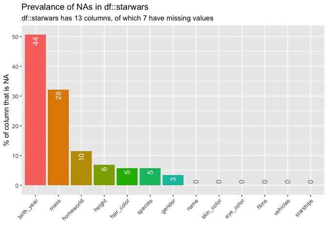
inspect_na() summarises the prevalence of missing values by each
column in a data frame. A tibble containing the count (cnt) and the
overall percentage (pcnt) of missing values is returned A barplot is
also returned when show_plot is set to TRUE.
inspect_na(starwars, show_plot = TRUE)## # A tibble: 13 x 3
## col_name cnt pcnt
## <chr> <int> <dbl>
## 1 birth_year 44 50.6
## 2 mass 28 32.2
## 3 homeworld 10 11.5
## 4 height 6 6.90
## 5 hair_color 5 5.75
## 6 species 5 5.75
## 7 gender 3 3.45
## 8 name 0 0
## 9 skin_color 0 0
## 10 eye_color 0 0
## 11 films 0 0
## 12 vehicles 0 0
## 13 starships 0 0
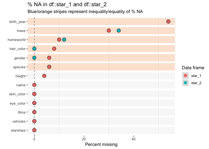
When a second dataframe is provided, inspect_na() returns a tibble
containing counts and percentage missingness by column, with summaries
for the first and second data frames are show in columns with names
appended with _1 and _2, respectively. In addition, a (p)-value is
calculated which provides a measure of evidence of whether the
difference in missing values is significantly different.
inspect_na(star_1, star_2, show_plot = TRUE)## # A tibble: 13 x 6
## col_name cnt_1 pcnt_1 cnt_2 pcnt_2 p_value
## <chr> <int> <dbl> <int> <dbl> <dbl>
## 1 birth_year 27 54 27 54 1
## 2 mass 15 30 17 34 0.830
## 3 homeworld 5 10 6 12 1.000
## 4 hair_color 4 8 0 0 0.126
## 5 gender 3 6 0 0 0.241
## 6 species 3 6 3 6 1
## 7 height 2 4 NA NA NA
## 8 name 0 0 NA NA NA
## 9 skin_color 0 0 0 0 NA
## 10 eye_color 0 0 0 0 NA
## 11 films 0 0 0 0 NA
## 12 vehicles 0 0 0 0 NA
## 13 starships 0 0 0 0 NA
Notes:
- Smaller (p)-values indicate stronger evidence of a difference in the missingness rate for a single column
- If a column appears in one data frame and not the other - for
example
heightappears instar_1but norstar_2, then the correspondingpcnt_,cnt_andp_valuecolumns will containNA - Where the missingness is identically 0, the
p_valueisNA. - The visualisation illustrates the significance of the difference
using a coloured bar overlay. Orange bars indicate evidence of
equality or missingness, while blue bars indicate inequality. If a
p_valuecannot be calculated, no coloured bar is shown. - The significance level can be specified using the
alphaargument toinspect_na(). The default isalpha = 0.05.
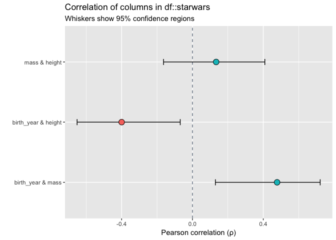
inspect_cor() returns a tibble containing Pearson’s correlation
coefficient, confidence intervals and (p)-values for pairs of numeric
columns . The function combines the functionality of cor() and
cor.test() in a more convenient wrapper. A point and whiskers plot is
also returned when show_plot = TRUE.
inspect_cor(starwars, show_plot = T)## # A tibble: 3 x 6
## col_1 col_2 corr p_value lower upper
## <chr> <chr> <dbl> <dbl> <dbl> <dbl>
## 1 birth_year mass 0.478 0.00318 0.130 0.721
## 2 birth_year height -0.400 0.00789 -0.651 -0.0690
## 3 mass height 0.134 0.312 -0.163 0.409
Notes
- The tibble is sorted in descending order of the absolute coefficient (|\rho|).
inspect_cordrops missing values prior to calculation of each correlation coefficient.- The
p_valueis associated with the null hypothesis (H_0: \rho = 0).
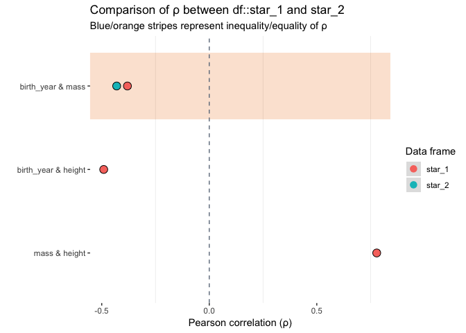
When a second dataframe is provided, inspect_cor() returns a tibble
that compares correlation coefficients of the first dataframe to those
in the second. The p_value column contains a measure of evidence for
whether the two correlation coefficients are equal or not.
inspect_cor(star_1, star_2, show_plot = TRUE)## # A tibble: 3 x 5
## col_1 col_2 corr_1 corr_2 p_value
## <chr> <chr> <dbl> <dbl> <dbl>
## 1 mass height 0.779 NA NA
## 2 birth_year height -0.491 NA NA
## 3 birth_year mass -0.381 -0.431 0.772
Notes:
- Smaller
p_valueindicates stronger evidence against the null hypothesis (H_0: \rho_1 = \rho_2) and an indication that the true correlation coefficients differ. - The visualisation illustrates the significance of the difference
using a coloured bar overlay. Orange bars indicate evidence of
equality of correlations, while blue bars indicate inequality. If a
p_valuecannot be calculated, no coloured bar is shown. - The significance level can be specified using the
alphaargument toinspect_cor(). The default isalpha = 0.05.
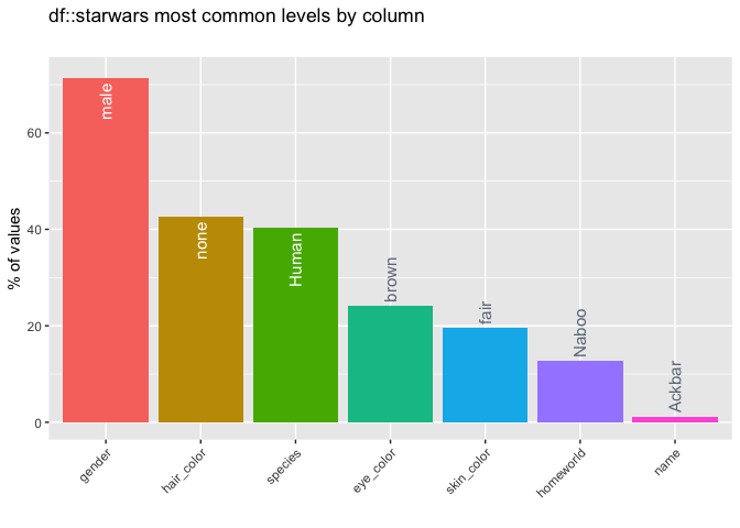
Understanding categorical columns that are dominated by a single level
can be useful. inspect_imb() returns a tibble containing categorical
column names (col_name); the most frequently occurring categorical
level in each column (value) and pctn & cnt the percentage and
count which the value occurs. The tibble is sorted in descending order
of pcnt. A barplot is also returned when show_plot is set to TRUE.
inspect_imb(starwars, show_plot = TRUE)## # A tibble: 7 x 4
## col_name value pcnt cnt
## <chr> <chr> <dbl> <int>
## 1 gender male 71.3 19
## 2 hair_color none 42.5 1
## 3 species Human 40.2 1
## 4 eye_color brown 24.1 10
## 5 skin_color fair 19.5 2
## 6 homeworld Naboo 12.6 3
## 7 name Ackbar 1.15 1
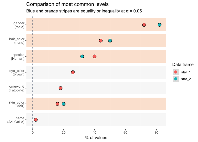
When a second dataframe is provided, inspect_imb() returns a tibble
that compares the frequency of the most common categorical values of the
first dataframe to those in the second. The p_value column contains a
measure of evidence for whether the true frequencies are equal or not.
inspect_imb(star_1, star_2, show_plot = TRUE)## # A tibble: 7 x 7
## col_name value pcnt_1 cnt_1 pcnt_2 cnt_2 p_value
## <chr> <chr> <dbl> <int> <dbl> <int> <dbl>
## 1 gender male 72 10 82 7 0.594
## 2 hair_color none 44 6 50 1 0.117
## 3 species Human 40 1 32 1 1
## 4 eye_color brown 26 7 NA NA NA
## 5 homeworld Tatooine 18 3 NA NA NA
## 6 skin_color fair 16 1 20 1 1
## 7 name Adi Gallia 2 1 NA NA NA
- Smaller
p_valueindicates stronger evidence against the null hypothesis that the true frequency of the most common values is the same. - The visualisation illustrates the significance of the difference
using a coloured bar overlay. Orange bars indicate evidence of
equality of the imbalance, while blue bars indicate inequality. If a
p_valuecannot be calculated, no coloured bar is shown. - The significance level can be specified using the
alphaargument toinspect_imb(). The default isalpha = 0.05.
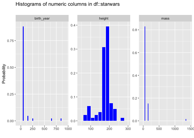
inspect_num() combining some of the functionality of summary() and
hist() by returning summaries of numeric columns. inspect_num()
returns standard numerical summaries (min, q1, mean,
median,q3, max, sd), but also the percentage of missing entries
(pcnt_na) and a simple histogram (hist). If show_plot = TRUE a
histogram is generated for each numeric feature.
inspect_num(starwars, show_plot = TRUE, breaks = 10)## # A tibble: 3 x 10
## col_name min q1 median mean q3 max sd pcnt_na hist
## <chr> <dbl> <dbl> <dbl> <dbl> <dbl> <dbl> <dbl> <dbl> <list>
## 1 birth_year 8 35 52 87.6 72 896 155. 50.6 <tibble [1…
## 2 height 66 167 180 174. 191 264 34.8 6.90 <tibble [1…
## 3 mass 15 55.6 79 97.3 84.5 1358 169. 32.2 <tibble [1…
The hist column is a list whose elements are tibbles each containing
the relative frequencies of bins for each feature. These tibbles are
used to generate the histograms when show_plot = TRUE. For example,
the histogram for starwars$birth_year is
inspect_num(starwars)$hist$birth_year## # A tibble: 20 x 2
## value prop
## <chr> <dbl>
## 1 [-Inf, 0) 0
## 2 [0, 50) 0.488
## 3 [50, 100) 0.395
## 4 [100, 150) 0.0465
## 5 [150, 200) 0
## 6 [200, 250) 0.0233
## 7 [250, 300) 0
## 8 [300, 350) 0
## 9 [350, 400) 0
## 10 [400, 450) 0
## 11 [450, 500) 0
## 12 [500, 550) 0
## 13 [550, 600) 0
## 14 [600, 650) 0.0233
## 15 [650, 700) 0
## 16 [700, 750) 0
## 17 [750, 800) 0
## 18 [800, 850) 0
## 19 [850, 900) 0.0233
## 20 [900, Inf) 0
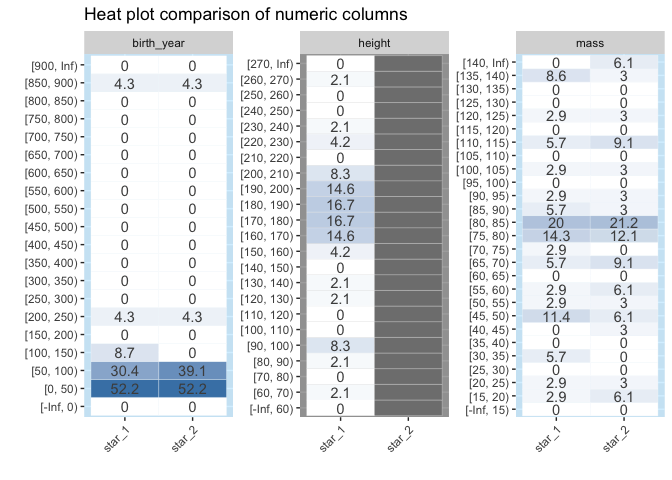
When comparing a pair of dataframes using inspect_num(), the
histograms of common numeric features are calculated, using identical
bins. The list columns hist_1 and hist_2 contain the histograms of
the features in the first and second dataframes. A formal statistical
comparison of each pair of histograms is calculated using Fisher’s exact
test, the resulting p value is reported in the column fisher_p.
When show_plot = TRUE, heat plot comparisons are returned for each
numeric column in each dataframe. Where a column is present in only one
of the dataframes, grey cells are shown in the comparison. The
significance of Fisher’s test is illustrated by coloured vertical bands
around each plot: if the colour is grey, no p value could be
calculated, if blue, the histograms are not found to be significantly
different otherwise the bands are red.
inspect_num(star_1, star_2, show_plot = TRUE)## # A tibble: 3 x 5
## col_name hist_1 hist_2 jsd fisher_p
## <chr> <list> <list> <dbl> <dbl>
## 1 birth_year <tibble [20 × 2]> <tibble [20 × 2]> 0.0474 0.354
## 2 height <tibble [23 × 2]> <NULL> NA NA
## 3 mass <tibble [27 × 2]> <tibble [27 × 2]> 0.122 0.694
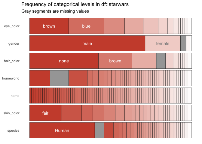
inspect_cat() returns a tibble summarising categorical features in a
data frame, combining the functionality of the inspect_imb() and
table() functions. If show_plot = TRUE a barplot is generated
showing the relative split. The tibble generated contains the columns
col_namename of each categorical columncntthe number of unique levels in the featurecommonthe most common level (see alsoinspect_imb())common_pcntthe percentage occurrence of the most dominant levellevelsa list of tibbles each containing frequency tabulations of all levels
inspect_cat(starwars, show_plot = T)## # A tibble: 7 x 5
## col_name cnt common common_pcnt levels
## <chr> <int> <chr> <dbl> <list>
## 1 eye_color 15 brown 24.1 <tibble [15 × 2]>
## 2 gender 5 male 71.3 <tibble [5 × 2]>
## 3 hair_color 13 none 42.5 <tibble [13 × 2]>
## 4 homeworld 49 Naboo 12.6 <tibble [49 × 2]>
## 5 name 87 Ackbar 1.15 <tibble [87 × 2]>
## 6 skin_color 31 fair 19.5 <tibble [31 × 2]>
## 7 species 38 Human 40.2 <tibble [38 × 2]>
For example, the levels for the hair_color column are
inspect_cat(starwars)$levels$hair_color## # A tibble: 13 x 2
## value prop
## <chr> <dbl>
## 1 none 0.425
## 2 brown 0.207
## 3 black 0.149
## 4 <NA> 0.0575
## 5 white 0.0460
## 6 blond 0.0345
## 7 auburn 0.0115
## 8 auburn, grey 0.0115
## 9 auburn, white 0.0115
## 10 blonde 0.0115
## 11 brown, grey 0.0115
## 12 grey 0.0115
## 13 unknown 0.0115
Note that by default, if NA values are present, they are counted as a
distinct categorical level.
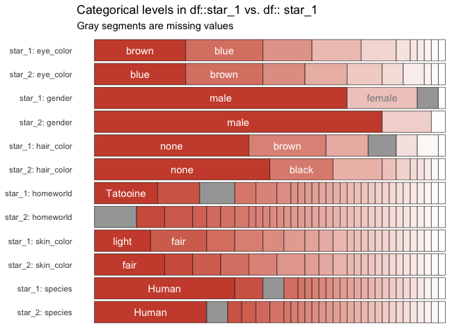
When two dataframes are compared using inspect_cat(), list columns are
returned for categorical columns common to both: lvls_1 and lvl2_2.
In addition, the Jensen-Shannon divergence (jsd) and p values
associated with Fisher’s exact test (fisher_p) are returned to enable
comparison of the distribution of levels in each pair of columns.
inspect_cat(star_1, star_2, show_plot = TRUE)## # A tibble: 7 x 5
## col_name jsd fisher_p lvls_1 lvls_2
## <chr> <dbl> <dbl> <list> <list>
## 1 eye_color 0.0817 0.785 <tibble [11 × 2]> <tibble [10 × 2]>
## 2 gender 0.0386 0.276 <tibble [4 × 2]> <tibble [3 × 2]>
## 3 hair_color 0.0951 0.418 <tibble [7 × 2]> <tibble [10 × 2]>
## 4 homeworld 0.282 0.998 <tibble [28 × 2]> <tibble [35 × 2]>
## 5 name NA NA <tibble [50 × 2]> <NULL>
## 6 skin_color 0.176 0.996 <tibble [23 × 2]> <tibble [23 × 2]>
## 7 species 0.161 1 <tibble [25 × 2]> <tibble [29 × 2]>
When show_plot = TRUE, a barplot is returned comparing distributions
of levels in pairs of columns shared by the two dataframes.

