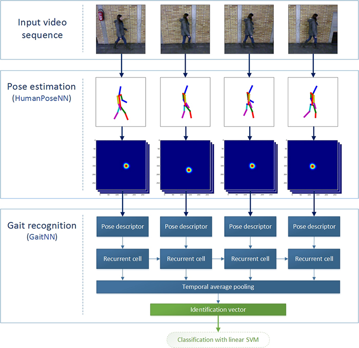
In this project you can find implementation of deep neural network for people identification from video by the characteristic of their gait. The processing is very robust against various covariate factors such as clothing, carrying conditions, shoe types and so on. Feel free to use this network in your project or extend it in some way.
The code was written in Python 3.5, but it is probably also compatible with other versions.
TensorFlow 1.3- how to install (however, some parts of code may be compatible with lower version, report an issue if you would have any problems.)numpy,scipy,PIL
The network takes raw RGB video frames of a pedestrian as an input and produces one-dimensional vector - gait descriptor that exposes as an identification vector. The identification vectors from gaits of each two different people should be linearly separable. Whole network consists of two sub-networks connected in cascade - HumanPoseNN and GaitNN.
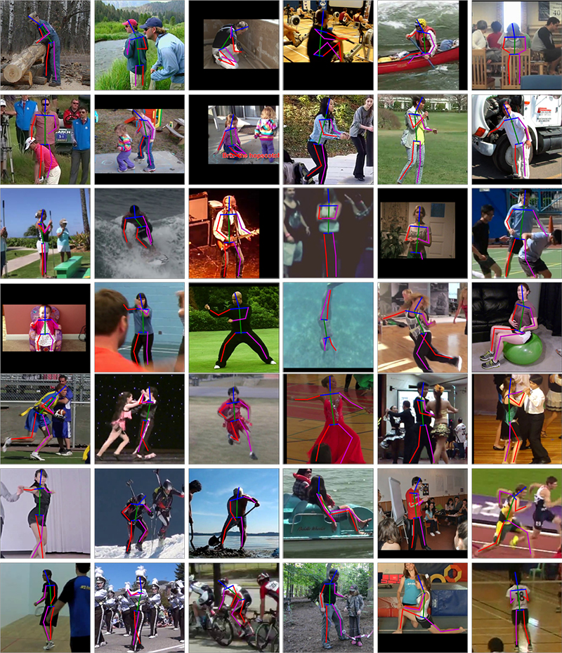
Spatial features from the video frames are extracted according to the descriptors that involve pose of the pedestrian. These descriptors are generated from the first sub-network - HumanPoseNN defined in human_pose_nn module. HumanPoseNN can be also used as a standalone network for regular 2D pose estimation problem from still images (for more info see this section).
Responsibility of the second sub-network - GaitNN defined in gait_nn module is the further processing of the generated spatial features into one-dimensional pose descriptors with the use of a residual convolutional network. Temporal features are then extracted across these pose descriptors with the use of the multilayer recurrent cells - LSTM or GRU. All temporal features are finally aggregated with Average temporal pooling into one-dimensional identification vector with good discriminatory properties. As already mentioned in the text above, the human identification vectors are linearly separable with each other and can therefore be classified with e.g. linear SVM.
The dummy code bellow shows how to generate the identification vector form the input data video_frames. For the best results, all frames should include the whole person visible from the profile view. The person should be located approximately in the center of each frame.
# Initialize computational graphs of both sub-networks
net_pose = HumanPoseIRNetwork()
net_gait = GaitNetwork(recurrent_unit = 'GRU', rnn_layers = 2)

# Load pre-trained models
net_pose.restore('path/to/pose_checkpoint.ckpt')
net_gait.restore('path/to/gait_checkpoint.ckpt')

# Create features from input frames in shape (TIME, HEIGHT, WIDTH, CHANNELS)
spatial_features = net_pose.feed_forward_features(video_frames)

# Process spatial features and generate identification vector
identification_vector = net_gait.feed_forward(spatial_features)The first sub-network HumanPoseNN can be also used as a standalone network for 2D pose estimation problem. This can be done in such a way:
net_pose = HumanPoseIRNetwork()

# Restore pre-trained model
net_pose.restore('path/to/pose_checkpoint.ckpt')

# input_images should contain RGB images (299 x 299) to be processed.
# The images in batch should be stacked along the first dimension, so the shape of input_images
# has to be (BATCH, 299, 299, 3)
coords_y, coords_x, probabilities = net_pose.joint_positions(input_images)
where coords_y, coords_x and probabilities stores estimated joint coordinates in Y axis, X axis and probability of each estimate, respectively. All these tensors have shape (BATCH, 16), where the second dimension is the body joint. The order of the body joints in the second dimension is as follows:
1. right ankle
2. right knee
3. right hip
4. left hip
5. left knee
6. left ankle
7. pelvis
8. thorax
9. upper neck
10. head top *(in human3.6m - head middle)*
11. right wrist
12. right elbow
13. right shoulder
14. left shoulder
15. left elbow
16. left wrist
If you want to get raw heat-maps mapping dense probability distribution for each pixel in image, use method heat_maps instead of method joint_positions. This method returns heat maps with shape (BATCH, HEIGHT, WIDTH, 16).
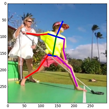
If you run the script dummy_pose_estimation.py, the pose of a human in the dummy image /images/dummy.jpg will be estimated and displayed in a new-created image /images/dummy_pose.jpg. For doing this you must have the matplotlib package installed and have pre-trained model MPII+LSP stored in /models/MPII+LSP.ckpt - for getting pre-trained models check the next section. The generated image in /images/dummy_pose.jpg should look like this one:
Printed probabilities of each estimate:
right ankle : 85.80%
right knee : 80.27%
right hip: 85.40%
left hip: 80.01%
left knee: 83.32%
left ankle: 92.08%
pelvis: 88.84%
thorax: 96.41%
upper neck: 97.40%
head top: 88.81%
right wrist: 87.90%
right elbow: 88.85%
right shoulder: 91.30%
left shoulder: 93.63%
left elbow: 92.31%
left wrist: 94.24%
Download: MPII+LSP.ckpt
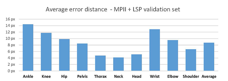
The checkpoint MPII+LSP.ckpt was trained on images from MPII and LSP database. In the graph below you can see the average distance between predicted and desired joints on a validation set of about 6 000 images.
Download: Human3.6m.ckpt (action walking)
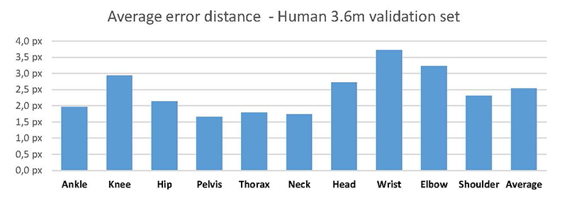
The checkpoint Human3.6m.ckpt was trained on the database Human 3.6m and only on the walking sequences of peoples S1, S6, S7, S8, S9 and S11 (48 sequences). Person S5 (8 sequences) was used for a validation purposes and the average distance between predicted and desired joints is shown in the following graph. As you can see, errors are smaller compared to MPII+LSP. It is because desired poses in Human 3.6m was labeled more precisely using motion capture system, so the a trained network can more accurately estimate the human pose. The second reason is that Human 3.6m sequences are very monotonous and thus human pose estimation is less challenging.
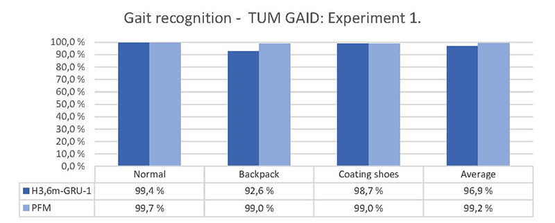
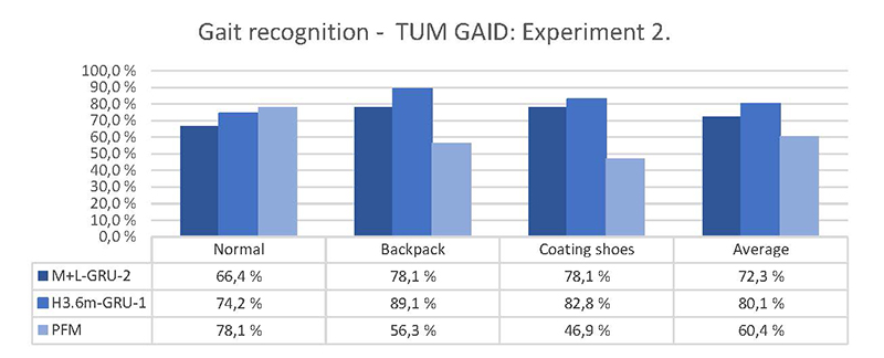
We use the same standard TUM GAID experiments as described e.g. in this paper (section Experimental results on TUM GAID) from F.M. Castro et al. that currently achieve state of the art results. In short, there are 2 main experiments. The goal in the first one is to identify 305 people (100 training, 150 validation, 155 testing) using 10 gait sequences for each person. These sequences catch person in three different covariate conditions: Normal walk, walking with backpack and walking with coating shoes. However, the people on all of these video-sequences wear the same clothing. To address the various clothing conditions, there is the second experiment. The goal of the second experiment is to identify 32 peoples (10 training, 6 validation, 16 testing) using 20 gait sequences for each person - first 10 was taken in January and the other 10 in April. The people have different clothing, usual for respective season.
The best performing model on the first experiment is H3.6m-GRU-1 and on the second is M+L-GRU-2. The graphs bellow compares the performance of these models with already mentioned state of the art model PFM from F.M. Castro et al. The model H3.6m-GRU-1 was trained only on the first experiment and on the second graph there is shown, how this model works on the validation set of the second experiment. As you can see, both models outperform PFM in the second experiment with a large margin. It means that these models are much more robust against clothing and time elapsed factors.
Download:
H3.6m-GRU-1.ckpt
M+L-GRU-2.ckpt
The name describe used architecture (model-RNNcell-layers), so e.g. checkpoint H3.6m-GRU-1.ckpt should be loaded in this way:
net_pose = HumanPoseIRNetwork()
net_gait = GaitNetwork(recurrent_unit = 'GRU', rnn_layers = 1)

# Load pre-trained models
net_pose.restore('./Human3.6m.ckpt')
net_gait.restore('./H3.6m-GRU-1.ckpt')