Interpretable Machine Learning with Python

Overview

Usage of AI and machine learning models is likely to become more commonplace as larger swaths of the economy embrace automation and data-driven decision-making. While these predictive systems can be quite accurate, they are usually treated as inscrutable black boxes that produce only numeric predictions with no accompanying explanations. Unfortunately, recent studies and recent events have drawn attention to mathematical and sociological flaws in prominent weak AI and ML systems, but practitioners don’t often have the right tools to pry open machine learning models and debug them. This series of notebooks introduces several approaches to that increase transparency, accountability, and trustworthiness in machine learning models. If you are a data scientist or analyst and you want to explain a machine learning model to your customers or managers (or if you have concerns about documentation, validation, or regulatory requirements), then this series of Jupyter notebooks is for you!

The notebooks highlight techniques such as:

The notebooks can be accessed through:

Enhancing Transparency in Machine Learning Models with Python and XGBoost - Notebook

Monotonicity constraints can turn opaque, complex models into transparent, and potentially regulator-approved models, by ensuring predictions only increase or only decrease for any change in a given input variable. In this notebook, I will demonstrate how to use monotonicity constraints in the popular open source gradient boosting package XGBoost to train a simple, accurate, nonlinear classifier on the UCI credit card default data.

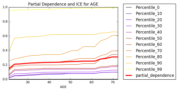
Once we have trained a monotonic XGBoost model, we will use partial dependence plots and individual conditional expectation (ICE) plots to investigate the internal mechanisms of the model and to verify its monotonic behavior. Partial dependence plots show us the way machine-learned response functions change based on the values of one or two input variables of interest, while averaging out the effects of all other input variables. ICE plots can be used to create more localized descriptions of model predictions, and ICE plots pair nicely with partial dependence plots. An example of generating regulator mandated reason codes from high fidelity Shapley explanations for any model prediction is also presented. The combination of monotonic XGBoost, partial dependence, ICE, and Shapley explanations is likely the most direct way to create an interpretable machine learning model today.

Increase Transparency and Accountability in Your Machine Learning Project with Python - Notebook

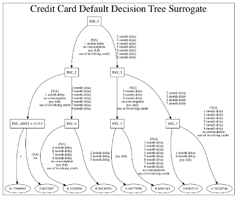
Gradient boosting machines (GBMs) and other complex machine learning models are popular and accurate prediction tools, but they can be difficult to interpret. Surrogate models, feature importance, and reason codes can be used to explain and increase transparency in machine learning models. In this notebook, we will train a GBM on the UCI credit card default data. Then we’ll train a decision tree surrogate model on the original inputs and predictions of the complex GBM model and see how the variable importance and interactions displayed in the surrogate model yield an overall, approximate flowchart of the complex model’s predictions. We will also analyze the global variable importance of the GBM and compare this information to the surrogate model, to our domain expertise, and to our reasonable expectations.

To get a better picture of the complex model’s local behavior and to enhance the accountability of the model’s predictions, we will use a variant of the leave-one-covariate-out (LOCO) technique. LOCO enables us to calculate the local contribution each input variable makes toward each model prediction. We will then rank the local contributions to generate reason codes that describe, in plain English, the model’s decision process for every prediction.

Explain Your Predictive Models to Business Stakeholders with LIME using Python and H2O - Notebook

Machine learning can create very accurate predictive models, but these models can be almost impossible to explain to your boss, your customers, or even your regulators. This notebook will use (Local Interpretable Model-agnostic Explanations) LIME to increase transparency and accountability in a complex GBM model trained on the UCI credit card default data. LIME is a method for building linear surrogate models for local regions in a data set, often single rows of data. LIME sheds light on how model predictions are made and describes local model mechanisms for specific rows of data. Because the LIME sampling process may feel abstract to some practitioners, this notebook will also introduce a more straightforward method of creating local samples for LIME.

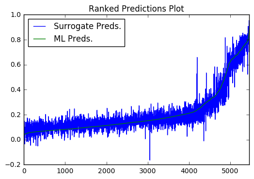
Once local samples have been generated, we will fit LIME models to understand local trends in the complex model’s predictions. LIME can also tell us the local contribution of each input variable toward each model prediction, and these contributions can be sorted to create reason codes -- plain English explanations of every model prediction. We will also validate the fit of the LIME model to enhance trust in our explanations using the local model’s R² statistic and a ranked predictions plot.

Testing Machine Learning Models for Accuracy, Trustworthiness, and Stability with Python and H2O - Notebook

Because machine learning model predictions can vary drastically for small changes in input variable values, especially outside of training input domains, sensitivity analysis is perhaps the most important validation technique for increasing trust in machine learning model predictions. Sensitivity analysis investigates whether model behavior and outputs remain stable when input data is intentionally perturbed, or other changes are simulated in input data. In this notebook, we will enhance trust in a complex credit default model by testing and debugging its predictions with sensitivity analysis.

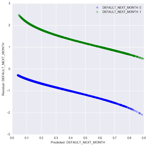
We’ll further enhance trust in our model using residual analysis. Residuals refer to the difference between the recorded value of a target variable and the predicted value of a target variable for each row in a data set. Generally, the residuals of a well-fit model should be randomly distributed, because good models will account for most phenomena in a data set, except for random error. In this notebook, we will create residual plots for a complex model to debug any accuracy problems arising from overfitting or outliers.

Using the Examples

O'Reilly Safari (recommended)

The ideal way to use these notebook is through O'Reilly Safari. Doing so will enable video narration by the notebook author and no installation of software packages is required. Individual lessons can be accessed below on Safari.

To use these notebooks outside of the Safari platform, follow the instructions below.

Docker Installation (recommended)

A Dockerfile is provided to build a docker container with all necessary packages and dependencies. This is the easiest way to use these examples if you are on Mac OS X, *nix, or Windows 10. To do so:

Install and start docker.

From a terminal:

Create a directory for the Dockerfile.
$ mkdir anaconda_py35_h2o_xgboost_graphviz
Fetch the Dockerfile.
$ curl https://raw.githubusercontent.com/jphall663/interpretable_machine_learning_with_python/master/anaconda_py35_h2o_xgboost_graphviz/Dockerfile > anaconda_py35_h2o_xgboost_graphviz/Dockerfile
Build a docker image from the Dockefile.
$ docker build anaconda_py35_h2o_xgboost_graphviz
Display docker image IDs. You are probably interested in the most recently created image.
$ docker images
Start the docker image and the Jupyter notebook server.
$ docker run -i -t -p 8888:8888 <image_id> /bin/bash -c "/opt/conda/bin/conda install jupyter -y --quiet && /opt/conda/bin/jupyter notebook --notebook-dir=/interpretable_machine_learning_with_python --ip='*' --port=8888 --no-browser"
Navigate to port 8888 on your machine, probably http://localhost:8888/.

Manual Installation

Anaconda Python 4.2.0 from the Anaconda archives along with the seaborn package.
Java.
The latest stable h2o Python package.
Git.
XGBoost with Python bindings.
GraphViz.

Anaconda Python, Java, Git, and GraphViz must be added to your system path.