yarox / data-eng-nano-project3

Code for the third project of the Udacity Data Engineering Nanodegree

Project 3: Data Warehouse

This is the code for the third project of the Udacity Data Engineering Nanodegree.

Project Overview

Introduction

A startup called Sparkify wants to analyze the data they've been collecting on songs and user activity on their new music streaming app. The analytics team is particularly interested in understanding what songs users are listening to. Their data resides in S3, in a directory of JSON logs on user activity on the app, as well as a directory with JSON metadata on the songs in their app.

We are going to build an ETL pipeline that extracts their data from S3, stages them in Redshift, and transforms the data into a set of fact and dimensional tables.

Schema Design

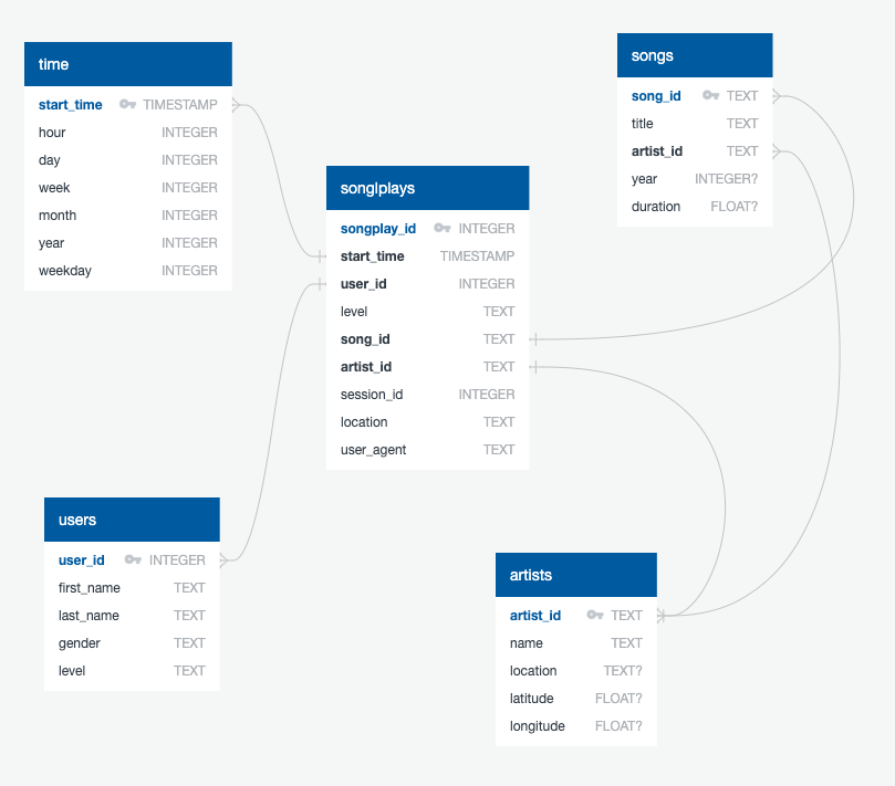
We created a star schema optimized for queries on song play analysis using the provided datasets. This includes the following tables.

Fact Table

1. songplays - records in log data associated with song plays i.e. records with page NextSong
   • songplay_id, start_time, user_id, level, song_id, artist_id, session_id, location, user_agent

Dimension Tables

1. users - users in the app

   • user_id, first_name, last_name, gender, level

2. songs - songs in music database

   • song_id, title, artist_id, year, duration

3. artists - artists in music database

   • artist_id, name, location, latitude, longitude

4. time - timestamps of records in songplays broken down into specific units

   • start_time, hour, day, week, month, year, weekday

ETL Pipeline

The pipeline is divided into creating the Redshift tables, loading the data into staging tables from S3 using COPY commands, and populating the final fact and dimension tables from the staging tables.

Quickstart

Project Structure

The project workspace includes these files:

• docker-compose.yml configures a Docker container for running the project.
• README.md

Under services/jupyter/config/src/:

• create_tables.py drops and creates the tables. Run this file to reset the tables before each time you run the ETL scripts.
• etl.py reads and processes files from song_data and log_data and loads them into the database.
• sql_queries.py contains all the sql queries.
• dashboard.ipynb displays a few example queries and results for song play analysis.
• dhw.cfg contains information about the Redshift cluster, the IAM role and the location of the S3 buckets.

Under services/jupyter/config/config/:

• requirements.txt holds the Python packages needed for this project.

Under services/jupyter/config/docker/:

• Dockerfile creates the Jupyter image we used for this project.

Amazon Web Services

The only things you need for running this code is an Redshift cluster up and running and an IAM role with AmazonS3ReadOnlyAccess permission attached to it in order for your cluster to load data from Amazon S3 buckets.

Get your cluster and role configuration from the AWS console and fill in the dwh.cfg file.

Running the code

We have two options for running the code: Docker containers or a local Python installation.

1. Docker

Make sure you have already installed both Docker Engine and Docker Compose. Everithing else is provided by the Docker images.

From the project directory, start up the application by running docker-compose up --build -d. Compose builds an image for the jupyter service, starts the container in the background, and leaves it running.

Execute docker-compose logs -f jupyter and check the server logs for a URL to connect to the notebook server.

To populate the tables open a Jupyter terminal, cd into the work directory, and run python create_tables.py followed by python etl.py. Remember to always run python create_tables.py before python etl.py in order to reset the database.

The file dashboard.ipynb provides example queries and results for song play analysis.

Execute docker-compose down to stop the container.

2. Local Installation

If you already have a Python installation on your system, check the dependencies from services/jupyter/config/requirements.txt and execute the code under services/jupyter/config/src/.

To populate the tables open a terminal, jump into the services/jupyter/config/src/ directory, and run python create_tables.py followed by python etl.py. Remember to always run python create_tables.py before python etl.py in order to reset the database.

Example Queries and Results

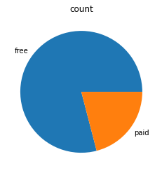
User Account Level

SELECT level, COUNT(*)
FROM users
GROUP BY level
ORDER BY level;

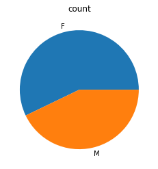
User Gender

SELECT gender, COUNT(*)
FROM users
GROUP BY gender
ORDER BY gender;

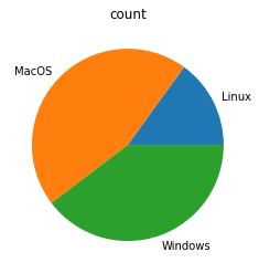
User Operating System

SELECT
    CASE
        WHEN user_agent LIKE '%Linux%' THEN 'Linux'
        WHEN user_agent LIKE '%Mac%' THEN 'MacOS'
        WHEN user_agent LIKE '%Windows%' THEN 'Windows'
        ELSE 'Unknown'
    END AS os,
    COUNT(*)
FROM
    songplays
GROUP BY os
ORDER BY os;

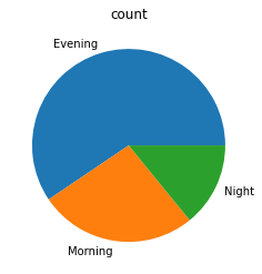
Most Popular Play Times Per Time of Day

SELECT
    CASE
        WHEN t.hour BETWEEN 6 AND 12 THEN 'Morning'
        WHEN t.hour BETWEEN 13 AND 22 THEN 'Evening'
        ELSE 'Night'
    END as result,
    COUNT(*)
FROM
    songplays AS s
    JOIN time AS t ON s.start_time = t.start_time
GROUP BY result
ORDER BY result;

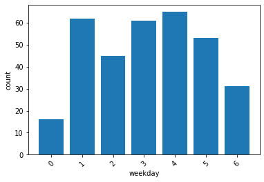
Most Popular Play Times Per Day of Week

SELECT
    t.weekday,
    COUNT(*)
FROM
    songplays AS s
    JOIN time AS t ON s.start_time = t.start_time
GROUP BY t.weekday
ORDER BY t.weekday;