wyniemko / Automated-Maintenance-Inspection-for-Amazon-Conveyor-Belts

Automate the inspection of conveyor belts by detecting tracking variances and surface defects (tears and stains).

Automated Maintenance Inspection for Amazon Conveyor Belts

The Conveyor Belt Monitoring System is an application that monitors the condition of a conveyor belt used in a manufacturing or logistics facility. The system uses computer vision to analyze images captured by a camera mounted above the conveyor belt. The system extracts key features such as the straightness of the belt, the number of rips on the belt, and the number of vertices on the belt surface. Based on these features, the system generates a report indicating the condition of the belt and whether maintenance is required.

Requirements

• Python 3.6 or higher
• Flask framework
• OpenCV 4.5 or higher
• NumPy 1.19 or higher
• SQLite 3

Running the Code

1. Clone the repository to your local machine.
2. Ensure that you have all the necessary packages installed. To do this, run pip install -r requirements.txt in your terminal or command prompt.
3. Open a new terminal or command prompt window and navigate to the directory where the code is located.
4. Run the run.py script by typing python run.py into the terminal or command prompt and pressing enter.
5. The program should start running, and you will see a message in the terminal or command prompt indicating that the web server is running.
6. Open a web browser and navigate to http://localhost:5000/ to view the home page of the web application.
7. Enter the required information on the home page and click the Start button to start the conveyor belt inspection process.
8. Once the inspection is complete, the results will be displayed on the results page. You can access the results page by clicking the View Previous Results button on the home page.
9. To view the data stored in the database, click the Data button on the home page to view a table of all previous inspection results.

Utilization of OpenCV Functions

• cv2.VideoCapture() – Captures video frames from a camera or a video file.
• cv2.cvtColor() – Converts an image from one color space to another.
• cv2.inRange() – Filters out pixels that are outside a specified range of values.
• cv2.findContours() – Detects contours (i.e., boundaries) of objects in an image.
• cv2.drawContours() – Draws contours onto an image.
• cv2.minAreaRect() – Finds the minimum bounding rectangle of a set of points.
• cv2.boxPoints() – Calculates the four corners of a rotated rectangle.

Main.py:

app = Flask(name)

• Initializes the Flask application.

@app.route('/', methods=['GET', 'POST'])

• Handles GET and POST requests for the index.html page.

def process_image(img)

• Processes a single image from the camera.
• Applies a series of image processing techniques to extract key features of the conveyor belt.
• Returns the extracted features.

@app.route('/process', methods=['POST'])

• Handles POST requests for the index.html page.
• Calls process_image() function to extract features from the image.
• Calculates average values for each feature across multiple images.
• Renders the results.html page with the calculated averages.

@app.route('/data')

• Handles GET requests for the data.html page.
• Queries the SQLite database for previous reports.
• Renders the data.html page with the retrieved reports.

@app.route('/update_benchmark_values', methods=['POST'])

• Handles POST requests for the results.html page.
• Updates the benchmark values used for comparison in the report.
• Redirects to the results.html page with updated benchmark values.

Part 0: Updates

All steps below have been integreated into a flask web server. A home page, belt maintenance report, and data page has been added.

Part 1: Video Capture

In the first part of the code, the user is prompted to enter the speed and length of a conveyor belt. The cycle length of the belt is then calculated using the formula:

cycle_length = length / speed * 5280 / 3600

The video codec used to compress the video file is set to mp4v using the cv2.VideoWriter_fourcc function. The total number of frames in the video is obtained using the cv2.VideoCapture.get function with the cv2.CAP_PROP_FRAME_COUNT argument. The images are read and written to files using the cv2.imread and cv2.imwrite functions, respectively. The recording stops after the calculated cycle length has elapsed.

Part 2: Frame Extraction

In this part, the video file is loaded using cv2.VideoCapture and the number of frames in the video is determined using cv2.CAP_PROP_FRAME_COUNT. The code then extracts the first 300 frames and saves them as individual JPG images in a folder named "Frame".

Part 3: Image Masking

This section of the code processes the images in the "Frame" folder by masking them using OpenCV's rectangle drawing and bitwise operations. To mask the images, a black image with the same size as the frame is created using mask = np.zeros((height, width, 3), np.uint8), and a white rectangle is drawn on the mask to cover everything outside of the middle square. The mask is then inverted and applied to the frame using the cv2.bitwise_and function.

Part 4: Vertical Belt Length Detection

Using two edge detection algorithms - Hough and Sobel - to detect the edges in the images.

Sobel Edge Detection

First, I extract the frames from the video and apply Sobel edge detection and Canny edge detection to the grayscale image. I then apply the Sobel edge detection on the Y-axis to detect vertical edges and save the resulting image in the "Edge" folder. The Sobel algorithm works by computing the gradient of the image using two linear operators, one for detecting horizontal edges and the other for detecting vertical edges. The output of the two convolutions is combined to create a single edge map that highlights areas of high intensity change in any direction. This edge map is thresholded to identify the edges in the original belt image.

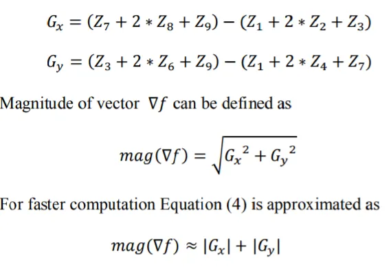
Using the Sobel edge detection method to detect edges in an image by computing the gradient of the image. This is done using two linear operators, one for detecting horizontal edges and the other for detecting vertical edges, which are applied to the image to obtain the gradient components in both directions.

Hough Transformation

Next, I use the Hough transformation algorithm to detect the straight lines in the image. The Hough transformation algorithm works by converting the image from Cartesian coordinates (x, y) to polar coordinates (r, θ) using the Hough transform. This transforms each point in the original image to a line in the transformed image.

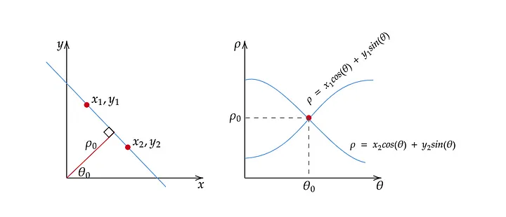
The Hough Space is now represented with ρ and θ instead of slope a and intercept b, where the horizontal axis is for the θ values and the vertical axis is for the ρ values. An edge point generates a cosine curve in the Hough Space, replacing the straight line representation and resolving the issue of unbounded values of a that arises when dealing with vertical lines.

The algorithm counts the number of intersections of lines in the transformed image, which correspond to points in the original image that are part of the same line. By thresholding the number of intersections, we can identify the lines in the original belt image.

After processing the images to grayscale with Sobel edge and Canny edge detection, I loop through each file in the "Edge" folder and apply the Hough transformation algorithm to detect the vertical lines in the image. I store the resulting value of the "straightness" in a list called "straightness_values".

Part 5: Material, Amnesty, Rip Defect Analysis

The detect_defects() function takes in a frame and an image name as input, which represent a single frame of a video feed and the name of the corresponding image file, respectively. The function then processes the frame to detect material defects, rip defects, and amnesty defects.

The first step in the function is to convert the input frame to grayscale using OpenCV's cvtColor() function. The grayscale image is stored in the variable gray.

The next step is to detect material defects in the frame. This is done by applying a binary threshold to the grayscale image. The threshold value of 200 is chosen to obtain a binary image with clear contrasts between the defects and the background. The threshold() function returns a thresholded image which is then used to find contours in the image using findContours() function. The contours represent the boundaries of the defects in the image. A loop then iterates over each contour and computes the area of the contour using the contourArea() function. If the area of the contour is greater than 500 pixels, it is considered a material defect and its count is incremented. The drawContours() function is then used to draw a red contour line around the defect in the original frame. The final count of material defects is stored in the variable material_count.

The next step is to detect rip defects in the frame. The Sobel operator is applied to the grayscale image in the x-direction using the Sobel() function. This generates an image highlighting the edges in the x-direction. The for loop then iterates over each column of the Sobel image and computes the difference between adjacent pixels in the column. When the difference is negative for one pixel and positive for the next pixel, a rip is detected. The circle() function is used to draw a green circle around the rip in the original frame. Additionally, a separate screenshot of the rip is saved to the 'Rip_defects' folder for further analysis. The final count of rip defects is stored in the variable rip_count.

The last step is to detect amnesty defects in the frame. The Sobel operator is applied to the grayscale image in the y-direction using the Sobel() function. This generates an image highlighting the edges in the y-direction. The for loop then iterates over each row of the Sobel image and computes the difference between adjacent pixels in the row. When the difference is positive for one pixel and negative for the next pixel, an amnesty is detected. The circle() function is used to draw a blue circle around the amnesty in the original frame. Additionally, a separate screenshot of the amnesty is saved to the 'Amnesty_defects' folder for further analysis. The final count of amnesty defects is stored in the variable amnesty_count.

The detect_defects() function then returns the original frame with all the detected defects highlighted, along with the counts of material, rip, and amnesty defects.

The main code segment first creates three output folders for material, rip, and amnesty defect screenshots using the os.makedirs() function. The images list is then populated with the names of all the images in the 'Defect_frames' folder that end with '.jpg'.

A for loop is then used to iterate over each image in the images list. Within the loop, the cv2.imread() function is used to read the image file as a frame. The detect_defects() function is then called to detect defects in the frame, and the resulting counts of material, rip, and amnesty defects are stored in material_count, rip_count, and amnesty_count, respectively. The output frame is also returned from the detect_defects function, which means it can be used for further analysis or processing. Additionally, the function saves screenshots of any detected rip or amnesty defects to separate folders, which can be useful for further inspection or documentation.

The code then creates three output folders for material, rip, and amnesty defects and saves the output image to the main output folder. It also prints out the counts of each type of defect for the current image.

Finally, the code loops through the counts of each type of defect and saves any corresponding defect screenshots to the appropriate output folder. If there were no defects of a particular type detected, no screenshot is saved for that type.

Conclusion

In conclusion, the presented code offers a straightforward solution for conducting various video analysis tasks utilizing OpenCV and Numpy. With the input of conveyor belt speed and length, the code is capable of automatically computing the cycle length and extracting essential frames for further analysis. The code efficiently applies masking and edge detection techniques to identify and measure the vertical length of the gray belt, making it a valuable tool for studying conveyor belt operations.

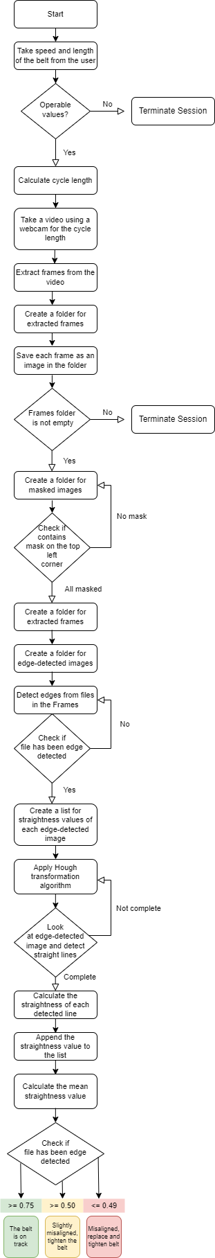
Flow-chart: order of operations